A Treemap is a graphical form used to represent heirarchical data. For example, population data may be gathered at the level of countries, and then aggregated to populations of entire continents. Figure 1, “A Treemap” shows a treemap of world population data with these two levels of aggregation (created with the treemap() function from the treemap package). The idea is that the plot is contained within a large rectangle, which is broken up into sub-rectangles to represent the populations of continents. Then each continent rectangle is further sub-divided into regions representing each individual country.

Figure 1. An example of a Treemap. The overall rectangle is broken into regions representing the population on each continent, then each continent region is further sub-divided to represent the population in each country. In this case, the treemap is further embellished by filling each region with a colour to indicate gross national income (per capita).

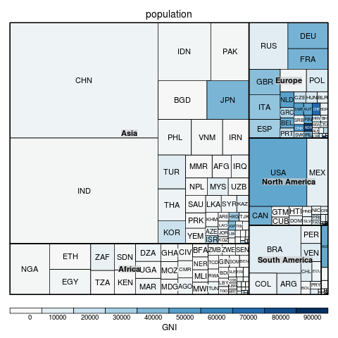Some limitations of Treemaps are that the sub-divided regions can become very thin (though this can be ameliorated with a "Squarified" Treemap), higher-level cell boundaries can be confused with lower-level cell boundaries (because all boundaries are vertical or horizontal lines), and Treemaps do not adapt well to non-rectangular regions.

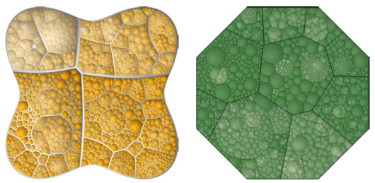
A Voronoi Treemap is an alternative representation of hierarchical data that is based on non-rectangular regions and offers a possible resolution to some of the problems described above. In particular, with this representation, there is less chance of higher-level cell boundaries being confused with lower-level cell boundaries (because the cells boundaries are not all vertical or horizontal lines) and arbitrarily-shaped regions can be sub-divided (not just rectangular regions). Figure 2, “Voronoi Treemaps” shows two (colourful) examples.

Figure 2. Two examples of Voronoi Treemaps

Voronoi Treemaps have been used by the Federal Statistical Office of Germany to display the make up of the Consumer Price Index (CPI) and the New York Times to show how the United States Federal Reserve calculates its CPI. Figure 3, “The Price Kaleidoscope” shows the German CPI diagram which they call a "Price Kaleidoscope".

Figure 3. The Price Kaleidoscope

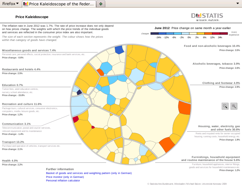
Statistics New Zealand, the national statistics office of New Zealand, expressed an interest in producing a Price Kaleidoscope for New Zealand's CPI data. However, neither the New York Times nor the German images provide a convenient basis for adapting to New Zealand CPI data. The New York Times figure is an Adobe Flash application, which would require special software to explore the underlying source code, assuming that permission were given to do so. The German figure is a combination of SVG and javascript, but the source file is protected by a copyright statement and would require considerable manual effort to adapt in any case.

This article describes the development of Open Source code to assist in the production of a Price Kaleidoscope for New Zealand CPI data. The focus in this article is on the production of the Voronoi Treemap that forms the basis of the Price Kaleidoscope.

the section called “Generating a Voronoi Treemap” briefly describes two high-level functions that can be used to generate a Voronoi Treemap. The subsequent sections look at the underlying code in much greater detail and point out some of the implementation details. A final section provides links to the complete code base. the section called “Generating a Voronoi Treemap” should contain sufficient information to be able to generate the information required to draw a Voronoi Treemap, with subsequent sections progressively more useful for people wanting to understand how the Treemap was generated or wanting to adapt the code to other purposes.

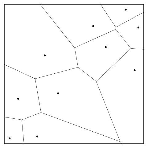
A (planar) Voronoi tessellation is based on a set of points in 2D space, hereafter called the sites. A Voronoi tessellation divides the 2D plane into non-overlapping regions, hereafter cells, such that any point in region i is closer to site i than to any other site.

As an example, the following R code generates 10 locations in the unit square and then uses the deldir() function from the deldir package to calculate a Voronoi Tesselation. The tessellation is plotted in Figure 4, “A Voronoi tessellation”.

library(deldir)
x <- 1000*runif(10)
y <- 1000*runif(10)
vt <- deldir(x, y)
png("tessellation.png")
par(mar=rep(1, 4))
plot(x, y, axes=FALSE, ann=FALSE, pch=16)
plot(vt, wlines="tess", lty="solid", add=TRUE)
box()
dev.off()

Figure 4. An example of a Voronoi tessellation

An (additively) weighted Voronoi tessellation is a generalisation where each site can also have a weight associated with it. This means that the distance of a point from each site becomes the normal Euclidean distance minus the weight of the site. The result is that the boundary of the region around each site consists of a set of hyperbolic curves rather than simple straight lines.

This article describes a function called awv() that uses the CGAL geometry library to generate an additively weighted Voronoi tessellation (see the section called “The awv() function” for more details). The following R code shows the function being used with the locations from Figure 4, “A Voronoi tessellation”, with some randomly-generated weights.

w <- runif(10, 1, 100)
library("gpclib")
unitSquare <- as(list(x=c(0, 0, 1000, 1000, 0),
                      y=c(0, 1000, 1000, 0, 0)),
                 "gpc.poly")
awvt <- awv(list(x=x, y=y), w, unitSquare)

The result of calling awv() is a list of polygons (technically, "gpc.poly" objects) that describe the Voronoi tessellation cells, which can be drawn simply by calling the plot() function. The following R code demonstrates this and Figure 5, “An additively weighted Voronoi tessellation” shows the result. The gpclib package is required to produce a bounding region for the tessellation and to draw the resulting cells for each site.

png("awv.png")
par(mar=rep(1, 4))
plot(x, y, axes=FALSE, ann=FALSE, pch=16)
lapply(awvt, plot, add=TRUE)
text(x, y, round(w), pos=3)
box()
dev.off()

Figure 5. An example of an additively weighted Voronoi tessellation. Each site has its weight shown as a text label

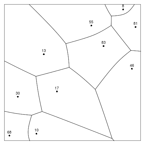A Voronoi Treemap (with a single level) can be used to represent a set of proportions that sum to 1 (e.g., the proportion of the World's population on each continent). A Voronoi Treemap consists of an additively weighted Voronoi tessellation, with the locations and weights of the sites selected so that the proportional area of each cell in the tessellation matches the set of target proportions being represented (e.g., if 40% of the World's population reside on continent i, then the area of cell i in the Voronoi Treemap will be 40% of the total region being tessellated).

The selection of appropriate site locations and weights proceeds iteratively, following the algorithm described in the article by Balzer and Deussen. Initial sites and weights are selected, an additively weighted Voronoi tessellation is generated, the areas of the cells in the tessellation are calculated, then the sites locations and weights are adjusted with the aim of improving the difference between the areas of the cells and the target proportions.

This algorithm is implemented by the function allocate() (see the section called “The allocate() function”). The R code below generates a set of target proportions and then calls allocate() to generate a Voronoi Treemap (with one level) that allocates subregions within the unit square corresponding to the target proportions. The final result is shown in Figure 6, “A Voronoi Treemap”, which was produced with the drawRegions() function (see the section called “Debugging Tools”). The starting point for this Treemap is the set of site locations and weights from Figure 5, “An additively weighted Voronoi tessellation”, but the locations and weights in the final result are very different. Figure 7, “A Voronoi Treemap animation” shows an animation of the iterative process that lead to the final result.

temp <- seq(.1, .9, length=10)
target <- temp/sum(temp)

treemap <- allocate(letters[1:10], 
                    list(x=x, y=y), 
                    w, unitSquare, target)
drawRegions(treemap, label=TRUE)

The result returned by allocate() is a list containing: a list of polygons that describe the cell boundaries; a list containing the locations of the sites; a vector of weights; a vector of cell areas; and the vector of target proportions. This information can be used to draw a Voronoi Treemap, for example using the drawRegions() function as above, or to generate further levels of Voronoi Treemap by further sub-dividing the cells. The following code prints out some of this information to demonstrate that the cells produced in the example above have areas that are very close to the target proportions.

area <- unlist(treemap$a)
temp <- rbind(100*round(area/sum(area), 3),
              100*round(target, 3))
colnames(temp) <- letters[1:10]
capture.output(temp)

[1] "     a   b   c   d   e    f    g    h    i  j"
[2] "[1,] 2 3.7 5.5 7.3 9.2 10.9 12.6 14.5 16.2 18"
[3] "[2,] 2 3.8 5.6 7.3 9.1 10.9 12.7 14.4 16.2 18"

Figure 6. An example of a Voronoi Treemap. A label has been drawn at each site location.

Figure 7. An animation of the Voronoi Treemap iterative process

The remaining sections of this document describe the underlying code in more detail.

The allocate() function is shown below. The additively weighted Voronoi tessellation is generated using the awv() function (see the section called “The awv() function”) and the subregion areas are calculated using area.poly() from gpclib. Testing showed that the algorithm sometimes failed to converge on a good solution, so that function also has a maxIterations argument to allow the function to give up after that many iterations. The debugging code is described in the section called “Debugging Tools”.

allocate

function (names, s, w, outer, target, maxIteration = 200, debug = FALSE, 
    dplot = FALSE, debugCell = FALSE) 
{
    count <- 1
    debugPlot <<- debugPlotGen()
    repeat {
        k <- awv(s, w, outer, debug, debugCell)
        areas <- lapply(k, area.poly)
        if (debug) {
            drawRegions(list(names = names, k = k, s = s, w = w, 
                a = areas, t = target), debug)
            info <- rbind(area = round(unlist(areas)/sum(unlist(areas)), 
                4), target = round(target, 4), weight = round(w, 
                1))
            colnames(info) <- names
            print(info)
        }
        if (count > maxIteration || breaking(unlist(areas), target, 
            debug = debug, dplot = dplot)) {
            return(list(names = names, k = k, s = s, w = w, a = areas, 
                t = target))
        }
        else {
            w <- adjustWeights(w, unlist(areas), target)
            s <- shiftSites(s, k)
            w <- shiftWeights(s, w)
        }
        count <- count + 1
    }
}

adjustWeights

function (w, a, target) 
{
    a <- ifelse(a == 0, 0.01 * sum(a), a)
    normA <- a/sum(a)
    w + mean(abs(w)) * ((target - normA)/target)
}

shiftSites

function (s, k) 
{
    newSites <- mapply(function(poly, x, y) {
        if (length(poly@pts)) {
            pts <- getpts(poly)
            TT.polygon.centroids(pts$x, pts$y)
        }
        else {
            c(x = x, y = y)
        }
    }, k, as.list(s$x), as.list(s$y), SIMPLIFY = FALSE)
    list(x = sapply(newSites, "[", "x"), y = sapply(newSites, 
        "[", "y"))
}

shiftWeights

function (s, w) 
{
    n <- length(s$x)
    for (i in 1:n) {
        for (j in 1:n) {
            if (i != j) {
                f = sqrt((s$x[i] - s$x[j])^2 + (s$y[i] - s$y[j])^2)/(abs(w[i]) + 
                  abs(w[j]))
                if (f > 0 && f < 1) {
                  w[i] <- w[i] * f
                  w[j] <- w[j] * f
                }
            }
        }
    }
    w
}

This section describes the code behind the awv() function that generates an additively weighted Voronoi tessellation. The main function itself consists of the following steps: write the site locations and weights out to an external file; do a system call to the external program voronoiDiagram; read the results of that external call from another external file; process the results to produce coherent region boundaries; then intersect the region boundaries with the overall region that is being divided up.

awv

function (s, w, region, debug = FALSE, debugCell = FALSE) 
{
    recordSites(s, w)
    result <- system("./voronoiDiagram > diagram.txt")
    if (result) 
        stop(paste("Voronoi diagram failed with error", result))
    roughCells <- readCells(s)
    tolerance <- 0.0015
    tidyCells <- tidyCells(roughCells, tolerance, debug, debugCell)
    trimCells(tidyCells, region)
}

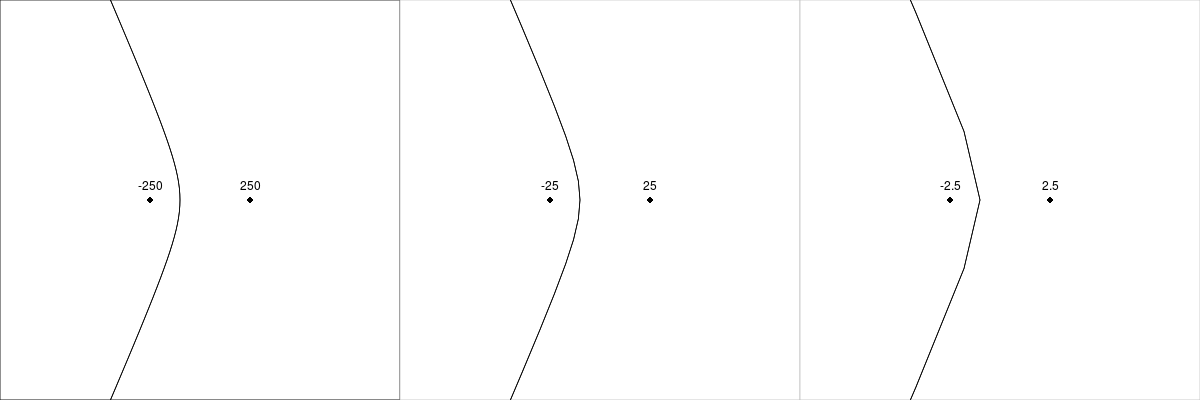
For best results, the site locations should be scaled so that they cover the range from -1000 to 1000. If site locations are given at a smaller scale, the curves produced for cell boundaries will be less smooth. Figure 8, “Scaling for site locations” shows the effect on the cell boundary for a simple case as site locations are scaled down. Initial weights should be assigned so that the largest is on the order of 100 (to correspond to the scaling for the site locations, but to still avoid overlaps between sites).

Figure 8. Diagrams showing the impact of different scales

The recordSites() function is simply a call to write.table(). The result is a file called sites.cin which is the input to the external program voronoiDiagram. A sample sites.cin file is shown in Figure 9, “A sample sites.cin file”.

recordSites

function (sites, weights) 
{
    write.table(cbind(sites$x, sites$y, weights), "sites.cin", 
        row.names = FALSE, col.names = FALSE)
}

-250 0 -100
250 0 100

The external program voronoiDiagram is described in more detail in the section called “The voronoiDiagram Program”. The result of calling this program is an external file called diagram.txt. Figure 10, “A sample diagram.txt file” shows an example.

Vertex -2.5 0
-1 0 -1.8 -3.42929
-1.8 -3.42929 -4.2 -9.34666
-4.2 -9.34666 -8.2 -18.6483
-8.2 -18.6483 -13.8 -31.5366
-13.8 -31.5366 -21 -48.0625
-21 -48.0625 -29.8 -68.2419
-29.8 -68.2419 -40.2 -92.0813
-40.2 -92.0813 -52.2 -119.583
-52.2 -119.583 -65.8 -150.749

readCells

function (s) 
{
    diagInfo <- readLines("diagram.txt")
    starts <- grep("^Vertex", diagInfo)
    lengths <- diff(c(starts, length(diagInfo) + 1))
    vertices <- read.table(textConnection(diagInfo[starts]))[-1]
    readCell <- function(start, length) {
        vline <- readLines("diagram.txt", n = start)[start]
        if (length > 1) {
            border <- read.table("diagram.txt", skip = start, 
                nrows = length - 1, na.strings = "nan")
        }
        else {
            border <- NULL
        }
        list(vertex = as.numeric(strsplit(vline, " ")[[1]][2:3]), 
            border = border)
    }
    result <- vector("list", length(s$x))
    for (i in 1:length(s$x)) {
        sx <- s$x[i]
        sy <- s$y[i]
        eps <- 0.01
        match <- which((abs(sx - vertices[, 1]) < eps) & (abs(sy - 
            vertices[, 2]) < eps))
        if (length(match)) {
            result[[i]] <- readCell(starts[match], lengths[match])
        }
        else {
            result[[i]] <- list(vertex = c(sx, sy), border = NULL)
        }
    }
    result
}

Tidying cell boundaries: the tidyCell() function

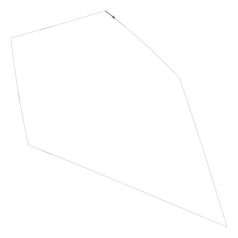
Unfortunately, the region boundaries from the file diagram.txt do not describe a contiguous set of line segments around the cell border. For example, Figure 11, “Drawing a boundary from the diagram.txt file” shows an animation that draws consecutive line segments for one of the cells in Figure 5, “An additively weighted Voronoi tessellation”. The segments describe the edges of the cell, but the edges are not drawn consecutively. (The segments actually backtrack sometimes as well, but that is less of a problem.)

Figure 11. An animation showing how the line segments from the diagram.txt do not form a single continuous border around the cell. These line segments have to be "tidied" to generate the vertices for a single polygon around the cell. (We can also see that the segments sometimes double back on themselves.) (Note that this example cell comes from the example additively weighted Voronoi tessellation shown in Figure 5, “An additively weighted Voronoi tessellation”.)

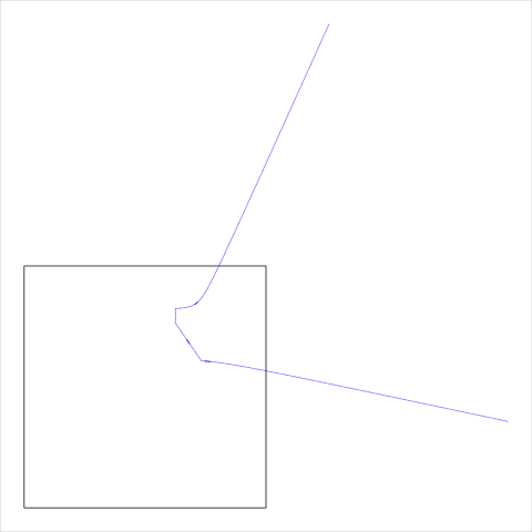
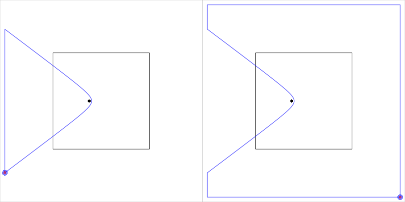
Another detail is that some cell borders are not closed (because the cell borders returned by voronoiDiagram are clipped to a rectangular region; see the section called “The voronoiDiagram Program”). Figure 12, “An open cell example” shows an example of an open cell.

Figure 12. An example of the sort of "open cell" that can be returned by voronoiDiagram. The black rectangle shows the overall region that is being tessellated and the semitransparent blue line shows the open cell boundary, which has been clipped to the larger white region. (Note that this example cell comes from the example additively weighted Voronoi tessellation shown in Figure 5, “An additively weighted Voronoi tessellation”.)

This means that the cell boundary information needs to be "tidied" so that we can use the segments to generate a set of vertices that describe a polygon around the cell. This job is performed by the tidyCells() function, which is itself simple because it passes most of the work on to the tidyCell() function.

+

tidyCells

function (cells, tolerance, debug = FALSE, debugCell = FALSE) 
{
    lapply(cells, tidyCell, tolerance, debug, debugCell)
}

The tidyCell() function in turn passes most of the real work of tidying up the cell boundary on to the getCellBorder() function. The purpose of the tidyCell() function is to handle the three possible results that can arise from tidying a cell boundary. The simplest case is that we have a closed cell, in which case the tidied boundary is returned. Another possibility is that we have an open cell. In that case, the cell needs to be closed; a job that is done by the closeCell() function. 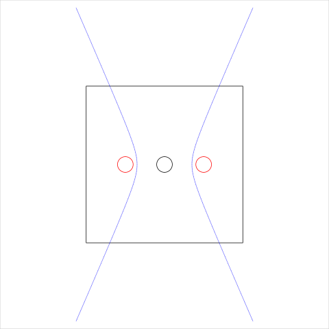The third, much more complex, possibility is that we have an open cell that consists of more than one open boundary.

Figure 13. An example of a "complex" open cell that consists of more than one open cell boundary. The black rectangle shows the overall region that is being tessellated and the semitransparent blue line shows the open cell boundaries, which have been clipped to the larger white region. The cell being described is the middle cell (containing the black circle), so the two open cell boundaries need to be connected at top and bottom to form a proper closed cell. The site locations used for this example are indicated by dots and the site weights are indicated by circles.

This sort of complex open cell is tidied by repeatedly called getCellBorder() until all open cell boundaries for a vertex have been extracted from the diagram.txt file. The result is a "multipleBorders" object that contains multiple lists (one for each open boundary). The simpler cases return just a single (open or closed) boundary as a normal list.

+

tidyCell

function (cell, tolerance, debug = FALSE, debugCell = FALSE) 
{
    if (debug && debugCell) 
        print(cell$vertex)
    border <- cell$border
    if (is.null(border)) 
        return(NULL)
    ok <- !apply(cell$border, 1, function(x) any(is.na(x)))
    border <- border[ok, ]
    result <- getCellBorder(border, tolerance = tolerance, debug = debug, 
        debugCell = debugCell)
    if (result$end == "boundary") {
        results <- list(result)
        repeat {
            result <- getCellBorder(border, seenBefore = result$seen, 
                tolerance = tolerance, debug = debug, debugCell = debugCell)
            if (result$end == "breakout") 
                break
            results <- c(results, list(result))
        }
        if (length(results) == 1) {
            result <- results[[1]]
        }
        else {
            result <- results
            class(result) <- "multipleBorders"
        }
    }
    if (inherits(result, "multipleBorders") || result$end == 
        "boundary") {
        cellBorder <- closeCell(result, cell$vertex, tolerance)
    }
    else {
        cellBorder <- list(x = c(result$x, result$x[1]), y = c(result$y, 
            result$y[1]))
    }
    cellBorder
}

The getCellBorder() function is quite long, but it implements a relatively simple algorithm: find a starting line segment, then find a line segment that follows on from that segment, then repeat until you get back to where you started.

In a little more detail, the first step is to find a starting line segment. For an open cell, this is one end of the cell boundary (where the boundary meets the larger clip region), otherwise it is just the first segment of the boundary. Having decided on a start segment (A), we look at the next segment (B) to see if segment B starts where segment A ended. We carry on as long as segments follow on from each other like this. When we hit a break, we look elsewhere in the set of segments for a segment that starts where the break left us (always ignoring segments that we have already used). If we cannot find any segment that starts at the right place, we look for a segment that ends at the right place (i.e., we look for a series of segments that arrives at the break point from the other direction). If we find such a segment, then we follow that segment backwards for as long as we keep finding contiguous segments.

The possible end conditions are: for an open cell, we hit the outer clip region again (the other end of the open cell boundary); for a closed cell, we get back to the point where the first segment started (we close the cell); we run out of segments. The second case gives us a finished cell boundary. The third result means that something is wrong, but we carry on by just joining the last point to the first point and issue a warning. The first result is good, but it requires further work to complete the cell boundary, and that is the job of the closeCell() function.

One detail about this algorithm is that a tolerance must be set to determine when two line segments really do start and end at the same location (checking for equality of real values is pointless). This tolerance has been set to a fixed value based on trial-and-error so the code is vulnerable to this value not being appropriate for all possible Voronoi tessellations.

+

getCellBorder

function (border, seenBefore = numeric(), tolerance, debug, debugCell) 
{
    N <- nrow(border)
    direction <- 1
    vx <- numeric(N)
    vy <- numeric(N)
    vcount <- 1
    complete <- FALSE
    endCondition <- FALSE
    returning <- length(seenBefore)
    visited <- rep(FALSE, N)
    start <- which(border[, 1] == -2 * scale | border[, 1] == 
        2 * scale | border[, 2] == -2 * scale | border[, 2] == 
        2 * scale)
    start <- start[!start %in% seenBefore]
    if (length(start)) {
        index <- start[1]
        startingX <- border[index, 1]
        startingY <- border[index, 2]
        seenBefore <- c(seenBefore, index)
    }
    else {
        start <- which(border[, 3] == -2 * scale | border[, 3] == 
            2 * scale | border[, 4] == -2 * scale | border[, 
            4] == 2 * scale)
        start <- start[!start %in% seenBefore]
        if (length(start)) {
            index <- start[1]
            direction <- -1
            startingX <- border[index, 3]
            startingY <- border[index, 4]
            seenBefore <- c(seenBefore, index)
        }
        else if (returning) {
            complete <- TRUE
            vx <- numeric()
            vy <- numeric()
            endCondition <- "breakout"
        }
        else {
            index <- 1
            startingX <- border[index, 1]
            startingY <- border[index, 2]
        }
    }
    while (!complete) {
        if (debug && debugCell) 
            cat(paste(index, direction, "\n"))
        if (direction > 0) {
            x1 <- 1
            y1 <- 2
            x2 <- 3
            y2 <- 4
        }
        else {
            x1 <- 3
            y1 <- 4
            x2 <- 1
            y2 <- 2
        }
        vx[vcount] <- border[index, x1]
        vy[vcount] <- border[index, y1]
        vcount <- vcount + 1
        visited[index] <- TRUE
        if (all(visited)) {
            complete <- TRUE
        }
        else {
            nextIndex <- index + direction
            endX <- border[index, x2]
            endY <- border[index, y2]
            startX <- border[nextIndex, x1]
            startY <- border[nextIndex, y1]
            if (nextIndex > 0 && nextIndex <= N && sim(endX, 
                startX, tolerance) && sim(endY, startY, tolerance)) {
                index <- nextIndex
            }
            else {
                newIndex <- startsAt(border, endX, endY, direction, 
                  tolerance)
                newIndex <- newIndex[!visited[newIndex]]
                if (length(newIndex)) {
                  index <- newIndex[1]
                }
                else {
                  direction <- -direction
                  newIndex <- startsAt(border, endX, endY, direction, 
                    tolerance)
                  newIndex <- newIndex[!visited[newIndex]]
                  if (length(newIndex)) {
                    index <- newIndex[1]
                  }
                  else {
                    complete <- TRUE
                    warning("Failed to trace cell")
                  }
                }
            }
        }
        endCondition <- stopping(border[index, x2], border[index, 
            y2], startingX, startingY, tolerance)
        if (endCondition == "boundary") {
            vx[vcount] <- border[index, x1]
            vx[vcount + 1] <- border[index, x2]
            vy[vcount] <- border[index, y1]
            vy[vcount + 1] <- border[index, y2]
            vcount <- vcount + 2
            seenBefore <- c(seenBefore, index)
            complete <- TRUE
        }
        else if (endCondition == "start") {
            complete <- TRUE
        }
    }
    list(x = vx[1:(vcount - 1)], y = vy[1:(vcount - 1)], end = endCondition, 
        seen = seenBefore)
}

The closeCell() function is used to finish tidying up an open cell. The function is generic, with a default method to handle normal lists and a method specifically for handling "multipleBorders" objects.

+

closeCell

function (cell, vertex, tol) 
{
    UseMethod("closeCell")
}

The default closeCell() method has a simple algorithm: start from one end of the open cell boundary (which is on the edge of the overall clip region), and follow the clip region boundary clockwise until we reach the other end of the open cell boundary. Check whether the site location is inside the polygon that we have generated. If it is not, complete the cell by going anti-clockwise around the clip region boundary instead (and check that the site location is now inside the polygon that we have generated; otherwise we have a problem). 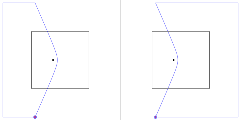Figure 14, “Closing an open cell” shows the two polygons that are generated by this algorithm for a simple test case.

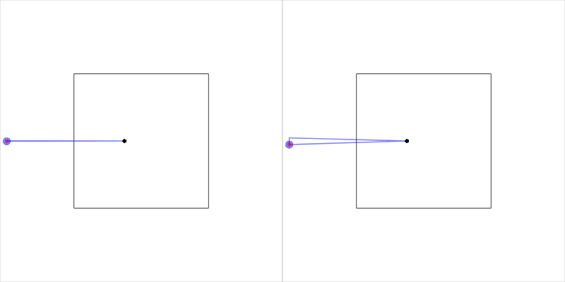
Figure 14. A diagram to illustrate the basic algorithm for closing open cells. Take the open cell boundary and join one end to the other by travelling clockwise around the clip region or by travelling anti-clockwise around the clip region. The solution is the closed cell that contains the site location.

The function is complicated by the need to handle a couple of special cases. The main special case occurs when an open cell starts and ends on the same edge of the clip region. In this case, the simple heuristic used to traverse the clip region boundary clockwise or anti-clockwise breaks down, so we first try just joining up the two end points. If that does not produce a polygon that contains the site location then we subtract that polygon from the entire clip region to produce the alternative cell boundary. Figure 15, “Closing an open cell” shows an example of this situation.

Figure 15. A diagram to illustrate the special case of closing an open cell when the two end points are on the same side of the clip region.

The other special case occurs when both end points of the open cell are identical. This produces a zero-area cell, which causes problems when we try to subtract this cell region from the clip region. The solution employed is to slightly "widen" the open cell by "stretching" the end points apart. Figure 16, “Closing an open cell” shows an example of this modification.

Figure 16. An example of an open cell when the two end points are identical. The closeCell() function expands the open cell by shifting the two end points apart.

It is also possible for the voronoiDiagram program to generate an open cell boundary where one end is not on the clip region boundary. This causes all sorts of problems, so if this situation is detected, the open cell is modified by adding a second end point identical to the first end point. This is a hack, pure and simple.

+

closeCell.default

function (cell, vertex, tol) 
{
    x <- cell$x
    y <- cell$y
    if (is.logical(cell$end)) {
        if (!cell$end) {
            x <- c(x, x[1])
            y <- c(y, y[1])
        }
    }
    N <- length(x)
    startSide <- side(x[1], y[1])
    endSide <- side(x[N], y[N])
    if (startSide == endSide) {
        if (sim(x[1], x[N], tol) && sim(y[1], y[N], tol)) {
            newx <- stretchX(x, y, N, startSide)
            newy <- stretchY(x, y, N, startSide)
            x <- newx
            y <- newy
        }
        cell <- list(x = c(x, x[1]), y = c(y, y[1]))
        if (point.in.polygon(vertex[1], vertex[2], cell$x, cell$y) == 
            0) {
            boundRect <- suppressWarnings(as(list(x = c(-2 * 
                scale, -2 * scale, 2 * scale, 2 * scale), y = c(-2 * 
                scale, 2 * scale, 2 * scale, -2 * scale)), "gpc.poly"))
            cellPoly <- suppressWarnings(as(cell, "gpc.poly"))
            cellPoly <- intersect(append.poly(cellPoly, boundRect), 
                boundRect)
            pts <- getpts(cellPoly)
            cell <- list(x = c(pts$x, pts$x[1]), y = c(pts$y, 
                pts$y[1]))
            if (point.in.polygon(vertex[1], vertex[2], cell$x, 
                cell$y) == 0) {
                stop("Failed to close cell")
            }
        }
    }
    else {
        cell <- closeClock(x, y, startSide, endSide)
        if (point.in.polygon(vertex[1], vertex[2], cell$x, cell$y) == 
            0) {
            cell <- closeAnti(x, y, startSide, endSide)
            if (point.in.polygon(vertex[1], vertex[2], cell$x, 
                cell$y) == 0) {
                stop("Failed to close cell")
            }
        }
    }
    cell
}

The closeCell() method for "multipleBorders" objects simply calls the default method for each border and produces an object of class "multipleCells", which is just a list of cells.

+

closeCell.multipleBorders

function (cell, vertex, tol) 
{
    result <- lapply(cell, closeCell, vertex, tol)
    class(result) <- "multipleCells"
    result
}

trimCells

function (cells, region) 
{
    polys <- lapply(cells, convertCell)
    lapply(polys, intersect, region)
}

convertCell

function (cell) 
{
    UseMethod("convertCell")
}

convertCell.default

function (cell) 
{
    if (is.null(cell)) {
        new("gpc.poly")
    }
    else {
        suppressWarnings(as(cell, "gpc.poly"))
    }
}

convertCell.multipleCells

function (cell) 
{
    polys <- suppressWarnings(lapply(cell, as, "gpc.poly"))
    Reduce(intersect, polys)
}

The external program that generates the additively weighted Voronoi tessellation is written in C++ and is based on the CGAL geometry library. The C++ code is shown below. The author is neither an expert in C++ nor in the CGAL library so there may be inefficiencies or clumsiness in this code.

/*
 *  Copyright (C) 2012 Paul Murrell
 *
 *  This program is free software; you can redistribute it and/or modify
 *  it under the terms of the GNU General Public License as published by
 *  the Free Software Foundation; either version 2 of the License, or
 *  (at your option) any later version.
 *
 *  This program is distributed in the hope that it will be useful,
 *  but WITHOUT ANY WARRANTY; without even the implied warranty of
 *  MERCHANTABILITY or FITNESS FOR A PARTICULAR PURPOSE.  See the
 *  GNU General Public License for more details.
 *
 *  You should have received a copy of the GNU General Public License
 *  along with this program; if not, a copy is available at
 *  http://www.gnu.org/licenses/gpl.txt
 */

// This code is based on a CGAL example 
// examples/Apollonius_graph_2/ag2_exact_traits.cpp

// standard includes
#include <iostream>
#include <fstream>
#include <cassert>

// the number type
#include <CGAL/MP_Float.h>


// example that uses an exact number type

#include <CGAL/Exact_predicates_inexact_constructions_kernel.h>
#include <CGAL/Delaunay_triangulation_2.h>
#include <iterator>

typedef CGAL::Exact_predicates_inexact_constructions_kernel K;
typedef K::Point_2 Point_2;
typedef K::Iso_rectangle_2 Iso_rectangle_2;
typedef K::Segment_2 Segment_2;
typedef K::Ray_2 Ray_2;
typedef K::Line_2 Line_2;

// typedefs for the traits and the algorithm

#include <CGAL/Apollonius_graph_2.h>
#include <CGAL/Apollonius_graph_traits_2.h>

typedef CGAL::Apollonius_graph_traits_2<K>   Traits;
typedef CGAL::Apollonius_graph_2<Traits>     Apollonius_graph;


//A class to recover Voronoi diagram from stream.
struct Cropped_voronoi_from_apollonius{
    std::list<Segment_2> m_cropped_vd;
    Iso_rectangle_2 m_bbox;
  
    Cropped_voronoi_from_apollonius(const Iso_rectangle_2& bbox):m_bbox(bbox){}
  
    template <class RSL>
    void crop_and_extract_segment(const RSL& rsl){
        CGAL::Object obj = CGAL::intersection(rsl,m_bbox);
        const Segment_2* s=CGAL::object_cast<Segment_2>(&obj);
        if (s) m_cropped_vd.push_back(*s);
    }
  
    void operator<<(const Ray_2& ray)    { crop_and_extract_segment(ray); }
    void operator<<(const Line_2& line)  { crop_and_extract_segment(line); }
    void operator<<(const Segment_2& seg){ crop_and_extract_segment(seg); }

    void reset() {
        m_cropped_vd.erase(m_cropped_vd.begin(), m_cropped_vd.end());
    }
};

int main()
{
  std::ifstream ifs("sites.cin");
  assert( ifs );

  Apollonius_graph ag;
  Apollonius_graph::Site_2 site;

  // read the sites and insert them in the Apollonius graph
  while ( ifs >> site ) {
    ag.insert(site);
  }

  //construct a rectangle
  // This is set up to be well outside the range of the sites
  // This means that we should be able to just join up the end
  // points for any open cells, without fear of crossing the 
  // area that contains the sites (EXCEPT for pretty pathological
  // cases, e.g., where there are only two sites)
  Iso_rectangle_2 bbox(-2000,-2000,2000,2000);

  Cropped_voronoi_from_apollonius vor(bbox);

  // iterate to extract Voronoi diagram edges around each vertex
  Apollonius_graph::Finite_vertices_iterator vit;
  for (vit = ag.finite_vertices_begin(); 
       vit != ag.finite_vertices_end(); 
       ++vit) {
      std::cout << "Vertex ";
      std::cout << vit->site().point();
      std::cout << "\n";
      Apollonius_graph::Edge_circulator ec = ag.incident_edges(vit), done(ec);
      if (ec != 0) {
          do { 
              ag.draw_dual_edge(*ec, vor);
              // std::cout << "Edge\n";
          } while(++ec != done); 
      }
      //print the cropped Voronoi diagram edges as segments
      std::copy(vor.m_cropped_vd.begin(),vor.m_cropped_vd.end(),
                std::ostream_iterator<Segment_2>(std::cout,"\n"));
      vor.reset();
  }

  //extract the entire cropped Voronoi diagram
  // ag.draw_dual(vor);

  return 0;
}

The code was based on one of the CGAL examples (ag2_exact_traits.cpp) and mainly consists of the creation of an Apollonius_graph object (based on sites recorded in the sites.cin file) followed by a call to the incident_edges method for each vertex in the Apollonius_graph (plus some code to crop the edges to a bounding region).

This program needs to be compiled into an executable for the platform on which the code will be run (it has only been tested on 3.2.0-27-generic #43-Ubuntu x86_64 x86_64 GNU/Linux). The compile will require the CGAL library to be installed; the CGAL manuals have good instructions (particularly Chapter 9).

This section describes some of the in-built debugging options that are available in this Voronoi Treemap implementation.

The allocate() function iteratively generates additively weighted Voronoi tessellations to attempt to produce a subdivision of the overall region that allocates a target proportion of the overall region to each subregion. This function does not always converge to an acceptable solution and it will simply stop after a fixed number of iterations. It is therefore useful to be able to check how well the function has performed.

A very simple test that the allocate() function has returned an acceptable result is to call the cellError() function, which returns the maximum difference between the cell area proportions and the target proportions. The following code demonstrates its use.

treemap <- allocate(letters[1:10], 
                    list(x=x, y=y), 
                    w, unitSquare, target)
cellError(unlist(treemap$a), treemap$t)

[1] 0.0006274598

To get a finer grained view of the performance of the allocate() function, the debug argument can be used to print out information about each iteration and this can be used to view the differences between the areas of allocated regions and the target values This also prints out the maximum cell error and site weights are also displayed. An example is shown below; this reports on the first few iterations for the Voronoi Treemap in Figure 6, “A Voronoi Treemap”. If the debug argument is TRUE, the additively weighted Voronoi tessellation is also drawn at each iteration (this produces a picture like the one in Figure 6, “A Voronoi Treemap”). The devAskNewPage()() function can be used to force a user prompt between each iteration.

temp <- capture.output(
treemap <- allocate(letters[1:10], 
                    list(x=x, y=y), 
                    w, unitSquare, target, 
                    maxIteration=2,
                    debug=TRUE)
)
temp

 [1] "             a       b       c      d       e       f       g       h       i"
 [2] "area    0.1033  0.1206  0.0652 0.0297  0.1173  0.0386  0.2339  0.0771  0.0693"
 [3] "target  0.0200  0.0378  0.0556 0.0733  0.0911  0.1089  0.1267  0.1444  0.1622"
 [4] "weight 17.1000 80.7000 29.7000 8.1000 55.3000 68.0000 45.7000 82.6000 10.0000"
 [5] "             j"                                                               
 [6] "area    0.1451"                                                               
 [7] "target  0.1800"                                                               
 [8] "weight 13.1000"                                                               
 [9] "Difference: 0.10719846042224 (0.106571000659323)"                             
[10] "               a       b       c       d       e       f       g        h"    
[11] "area      0.0026  0.0887  0.0768  0.0628  0.0918  0.0729  0.1777   0.2097"    
[12] "target    0.0200  0.0378  0.0556  0.0733  0.0911  0.1089  0.1267   0.1444"    
[13] "weight -153.7000 -9.2000 22.5000 32.5000 43.5000 94.5000 11.0000 101.7000"    
[14] "             i       j"                                                       
[15] "area    0.1013  0.1157"                                                       
[16] "target  0.1622  0.1800"                                                       
[17] "weight 33.5000 21.1000"                                                       
[18] "Difference: 0.0652576833869154 (0.0419407770353243)"                          
[19] "               a        b      c       d       e        f        g       h"   
[20] "area      0.0034   0.0535 0.0645  0.1056  0.0919   0.1092   0.1433  0.2038"   
[21] "target    0.0200   0.0378 0.0556  0.0733  0.0911   0.1089   0.1267  0.1444"   
[22] "weight -108.1000 -79.8000 2.6000 40.0000 43.1000 111.8000 -10.1000 78.1000"   
[23] "             i       j"                                                       
[24] "area    0.1118  0.1131"                                                       
[25] "target  0.1622  0.1800"                                                       
[26] "weight 53.1000 39.8000"                                                       

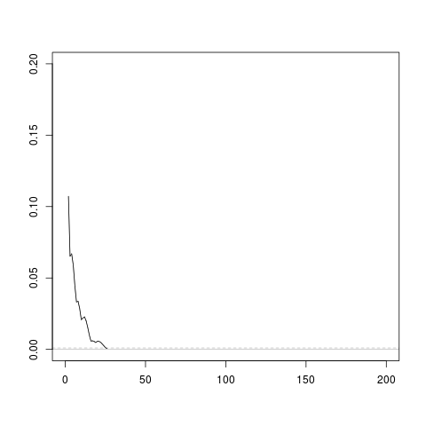
The dplot argument to the allocate() function can be used as an alternative to debug. If this argument is TRUE, a plot is drawn to show the error level at each iteration (the maximum difference between cell areas and target areas). Figure 17, “A debugging plot for allocate()” shows what this plot looks like for the Voronoi Treemap in Figure 6, “A Voronoi Treemap”.

Figure 17. An example of the debugging plot that is produced by the allocate() function when the dplot argument is TRUE. The line grows with each iteration and the iterations end when the line drops below the dashed grey line (or gets up to 200).

The arguments described above are useful for observing the progress of the allocate() function. There are also facilities that provide a more detailed view, which are helpful when the allocate() function either does not converge to an acceptable result or just fails altogether. One of these facilities is provided by the debugCell argument to the allocate() function. If this argument is TRUE then debugging output is produced by the getCellBorder() function to show the order in which segments from the diagram.txt file are being used to generate a cell border (plus the "direction" in which the cells are being followed). The output below shows an example of this output for the left cell in Figure 14, “Closing an open cell”. The first value shows that this is for the site vertex at location (-250, 0) and the remaining values show that the getCellBorder() function started at segment 32 (which is on the boundary of the clip region because this is an open cell), followed that backwards down to segment 1, then jumped to segment 33 and followed that (forwards) to the end of the file. These values are useful for further inspecting the diagram.txt file during debugging.

 [1] "[1] -250    0" "32 -1 "        "31 -1 "        "30 -1 "       
 [5] "29 -1 "        "28 -1 "        "27 -1 "        "26 -1 "       
 [9] "25 -1 "        "24 -1 "        "23 -1 "        "22 -1 "       
[13] "21 -1 "        "20 -1 "        "19 -1 "        "18 -1 "       
[17] "17 -1 "        "16 -1 "        "15 -1 "        "14 -1 "       
[21] "13 -1 "        "12 -1 "        "11 -1 "        "10 -1 "       
[25] "9 -1 "         "8 -1 "         "7 -1 "         "6 -1 "        
[29] "5 -1 "         "4 -1 "         "3 -1 "         "2 -1 "        
[33] "1 -1 "         "33 1 "         "34 1 "         "35 1 "        
[37] "36 1 "         "37 1 "         "38 1 "         "39 1 "        
[41] "40 1 "         "41 1 "         "42 1 "         "43 1 "        
[45] "44 1 "         "45 1 "         "46 1 "         "47 1 "        
[49] "48 1 "         "49 1 "         "50 1 "         "51 1 "        
[53] "52 1 "         "53 1 "         "54 1 "         "55 1 "        
[57] "56 1 "         "57 1 "         "58 1 "         "59 1 "        
[61] "60 1 "         "61 1 "         "62 1 "         "63 1 "        

Several functions are also provided for drawing diagrams during debugging. The drawRegion() function draws the bounding region within which allocation is occurring, the drawSites() function draws the location and weight for sites, the drawRoughCells() function can be used to draw the results from the readCells() function, and the drawTidyCells() function can be used to draw the results from the tidyCells() function. There is also a drawRegions() function that draws an entire allocate() result. All of these functions start a new page by default, but have a newpage argument that allows their output to be combined. Figure 12, “An open cell example” and Figure 13, “A complex open cell example” were both constructed using these functions.

This article describes R code (and C++ code) for two purposes:

This code can be used as a basis for generating a Voronoi Treemap with more than one level, such as a "Price Kaleidoscope" of CPI data.

The article also describes the algorithm behind the generation of Voronoi Treemaps and numerous details of this particular implementation.

There are several avenues for further exploration. Rather than having to call an external program, voronoiDiagram, to generate the additively weighted Voronoi tessellation, it would be more efficient to build a dynamic library and load and call that from R. It would be useful to explore the stability of the Voronoi Treemap algorithm more rigorously, in particular its dependence on some of the tweak parameters (such as the tolerance used to decide whether line segments are contiguous). An interesting extension would involve exploring different ways to generate the starting sites for the Voronoi Treemap (sites that begin adjacent to each other tend to end up adjacent to each other). For example, if cells are to be filled with a colour depending upon a covariate, it might be useful to select starting sites so that sites with similar covariate values are closer to each other. Finally, the code would be more useful and easier to share if it were bundled as an R package (though the CGAL dependency might introduce significant complexity, possibly requiring configuration code, particularly across different platforms).

This section contains links to the raw R code files. All code is free software, released under the GPL.