1.1 Case study: Point Nemo

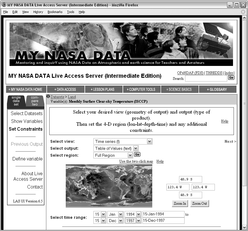
The Live Access Server is one of many services provided by the National Aeronautics and Space Administration (NASA) for gaining access to its enormous repositories of atmospheric and astronomical data. The Live Access Server^1.1provides access to atmospheric data from NASA's fleet of Earth-observing satellites, data that consist of coarsely gridded measurements of major atmospheric variables, such as ozone, cloud cover, pressure, and temperature. NASA provides a web site that allows researchers to select variables of interest, and geographic and temporal ranges, and then to download or view the relevant data (see Figure 1.1). Using this service, we can attempt to answer questions about atmospheric and weather conditions in different parts of the world.

The Pacific Pole of Inaccessibility is a location in the Southern Pacific Ocean that is recognized as one of the most remote locations on Earth. Also known as Point Nemo, it is the point on the ocean that is farthest from any land mass. Its counterpart, the Eurasian Pole of Inaccessibility, in northern China, is the location on land that is farthest from any ocean.

These two geographical extremes--one in the southern hemisphere, over 2,500 km from the nearest land, and one in the northern hemisphere, over 2,500 km from the nearest ocean--are usually only of interest either to intrepid explorers or conspiracy theorists (a remote location is the perfect place to hide an important secret!). However, our interest will be to investigate the differences in weather conditions between these interesting geographical extremes by using NASA's Live Access Server.

To make our task a little more manageable, for now we will restrict our attention to a comparison of the surface temperatures at each of the Poles of Inaccessibility. To be precise, we will look at monthly average temperatures at these locations from January 1994 to December 1997.

In a book on data analysis, we would assume that the data are already in a form that can be conveniently loaded into statistical software, and the emphasis would be on how to analyze these data. However, that is not the focus of this book. Here, we are interested in all of the steps that must be taken before the data can be conveniently loaded into statistical software.

As anyone who has worked with data knows, it often takes more time and effort to get the data ready than it takes to perform the data analysis. And yet there are many more books on how to analyze data than there are on how to prepare data for analysis. This book aims to redress that balance.

In our example, the main data collection has already occurred; the data are measurements made by instruments on NASA satellites. However, we still need to collect the data from NASA's Live Access Server. We will do this initially by entering the appropriate parameters on the Live Access Server web site. Figure 1.2 shows the first few lines of data that the Live Access Server returns for the surface temperature at Point Nemo.

**Figure 1.2:** The first few lines of plain text output from the Live Access Server for the surface temperature at Point Nemo.
VARIABLE : Mean TS from clear sky composite (kelvin) FILENAME : ISCCPMonthly_avg.nc FILEPATH : /usr/local/fer_data/data/ SUBSET : 48 points (TIME) LONGITUDE: 123.8W(-123.8) LATITUDE : 48.8S 123.8W 23 16-JAN-1994 00 / 1: 278.9 16-FEB-1994 00 / 2: 280.0 16-MAR-1994 00 / 3: 278.9 16-APR-1994 00 / 4: 278.9 16-MAY-1994 00 / 5: 277.8 16-JUN-1994 00 / 6: 276.1 ...

Figure 1.2: The first few lines of plain text output from the Live Access Server for the surface temperature at Point Nemo.

             VARIABLE : Mean TS from clear sky composite (kelvin)
             FILENAME : ISCCPMonthly_avg.nc
             FILEPATH : /usr/local/fer_data/data/
             SUBSET   : 48 points (TIME)
             LONGITUDE: 123.8W(-123.8)
             LATITUDE : 48.8S
                       123.8W 
                        23
 16-JAN-1994 00 /  1:  278.9
 16-FEB-1994 00 /  2:  280.0
 16-MAR-1994 00 /  3:  278.9
 16-APR-1994 00 /  4:  278.9
 16-MAY-1994 00 /  5:  277.8
 16-JUN-1994 00 /  6:  276.1
 ...

The first thing we should always do with a new data set is take a look at the raw data. Viewing the raw data is an important first step in becoming familiar with the data set. We should never automatically assume that the data are reliable or correct. We should always check with our own eyes. In this case, we are already in for a bit of a shock.

Anyone who expects temperatures to be in degrees Celsius will find values like 278.9 something of a shock. Even if we expect temperatures on the Fahrenheit scale, 278.9 is hotter than the average summer's day.

The problem of course is that these are scientific measurements, so the scale being used is Kelvin; the temperature scale where zero really means zero. 278.9 K is 5.8 $\ensuremath{^\circ}$ C or 42 $\ensuremath{^\circ}$ F, which is a cool, but entirely believable, surface temperature value. When planning a visit to Point Nemo, it would be a good idea to pack a sweater.

Looking at the raw data, we also see a lot of other information besides the surface temperatures. There are longitude and latitude values, dates, and a description of the variable that has been measured, including the units of measurement. This metadata is very important because it provides us with a proper understanding of the data set. For example, the metadata makes it clear that the temperature values are on the Kelvin scale. The metadata also tells us that the longitude and latitude values, 123.8 W and 48.8 S, are not exactly what we asked for. It turns out that the values provided by NASA in this data set have been averaged over a large area, so this is as good as we are going to get.

Before we go forward, we should take a step back and acknowledge the fact that we are able to read the data at all. This is a benefit of the storage format that the data are in; in this case, it is a plain text format. If the data had been in a more sophisticated binary format, we would need something more specialized than a common web browser to be able to view our data. In Chapter 5 we will spend a lot of time looking at the advantages and disadvantages of different data storage formats.

Having had a look at the raw data, the next step in familiarizing ourselves with the data set should be to look at some numerical summaries and plots. The Live Access Server does not provide numerical summaries and, although it will produce some basic plots, we will need a bit more flexibility. Thus, we will save the data to our own computer and load it into a statistical software package.

The first step is to save the data. The Live Access Server will provide an ASCII file for us, or we can just copy-and-paste the data into a text editor and save it from there. Again, we should appreciate the fact that this step is quite straightforward and is likely to work no matter what sort of computer or operating system we are using. This is another feature of having data in a plain text format.

Now we need to get the data into our statistical software. At this point, we encounter one of the disadvantages of a plain text format. Although we, as human readers, can see that the surface temperature values start on the ninth line and are the last value on each row (see Figure 1.2), there is no way that statistical software can figure this out on its own. We will have to describe the format of the data set to our statistical software.

In order to read the data into statistical software, we need to be able to express the following information: “skip the first 8 lines”; and “on each row, the values are separated by whitespace (one or more spaces or tabs)”; and “on each row, the date is the first value and the temperature is the last value (ignore the other three values)”. Here is one way to do this for the statistical software package R (Chapter 9 has much more to say about working with data in R):

This solution may appear complex, especially for anyone not experienced in writing computer code. Partly that is because this is complex information that we need to communicate to the computer and writing code is the best or even the only way to express that sort of information. However, the complexity of writing computer code gains us many benefits. For example, having written this piece of code to load in the data for the Pacific Pole of Inaccessibility, we can use it again, with only a change in the name of the file, to read in the data for the Eurasian Pole of Inaccessibility. That would look like this:

Imagine if we wanted to load in temperature data in this format from several hundred other locations around the world. Loading in such volumes of data would now be trivial and fast using code like this; performing such a task by selecting menus and filling in dialog boxes hundreds of times does not bear thinking about.

Going back a step, if we wanted to download the data for hundreds of locations around the world, would we want to fill in the Live Access Server web form hundreds of times? Most people would not. Here again, we can write code to make the task faster, more accurate, and more bearable.

As well as the web interface to the Live Access Server, it is also possible to make requests by writing code to communicate with the Live Access Server. Here is the code to ask for the temperature data from the Pacific Pole of Inaccessibility:

Again, that may appear complex, and there is a “start-up” cost involved in learning how to write such code. However, this is the only sane method to obtain large amounts of data from the Live Access Server. Chapters 7 and 9 look at extracting data sets from complex systems and automating tasks that would otherwise be tedious or impossible if performed by hand.

Writing code, as we have seen above, is the only accurate method of communicating even mildly complex ideas to a computer, and even for very simple ideas, writing code is the most efficient method of communication. In this book, we will always communicate with the computer by writing code. In Chapter 2 we will discuss the basic ideas of how to write computer code properly and we will encounter a number of different computer languages throughout the remainder of the book.

At this point, we have the tools to access the Point Nemo data in a form that is convenient for conducting the data analysis, but, because this is not a book on data analysis, this is where we stop. The important points for our purposes are how the data are stored, accessed, and processed. These are the topics that will be expanded upon and discussed at length throughout the remainder of this book.