 http://orcid.org/0000-0002-3224-8858
by Paul Murrell
http://orcid.org/0000-0002-3224-8858
Version 1: Tuesday 31 May 2022

This document
by Paul
Murrell is licensed under a Creative
Commons Attribution 4.0 International License.
This document describes developments in the
grobCoords() function in the R package 'grid', plus
improvements to the 'gridGeometry' package that makes use of
the grobCoords() function.
These features are available in R version 4.2.0 and in 'gridGeometry' version 0.3-0.
The grobCoords() function (introduced in R version 3.6.0)
generates a set of coordinates from a 'grid' grob.
For example, the following code defines a
'grid' rectangle grob (and draws it) then calculates
a set of coordinates
from this rectangle grob (the vertices of the rectangle).
The rectangle is centred 1 inch in from the
left of the image and 1 inch up form the bottom of the image
and is 1 inch square, so the vertices are at
(0.5, 0.5), (0.5, 1.5), (1.5, 1.5), and (1.5, 0.5).
library(grid)
rectangle <- rectGrob(1, 1, 1, 1, default.units = "in", name = "r")
grid.draw(rectangle)

coords <- grobCoords(rectangle, closed = TRUE)
coords
  grob r
    shape 1
      x: 0.5 0.5 1.5 ... [4 values]
      y: 0.5 1.5 1.5 ... [4 values]
The 'gridGeometry' package (Murrell, 2022a)
combines 'grid' grobs using
operators like "union" and "intersection".
For example, in the following code we define a triangle shape
(and draw it) then we call grid.polyclip() from 'gridGeometry'
to draw the union of the rectangle from above with this triangle.
library(gridGeometry)
triangle <- polygonGrob(c(1, 2, 2), c(1, 1.5, .5), default.units="in")
grid.draw(triangle)

grid.polyclip(rectangle, triangle, "union")

The 'gridGeometry' package works by getting coordinates for each
grob, via grobCoords(), and combining those coordinates
using the 'polyclip' package (Johnson and Baddeley, 2019).
Any changes to the grobCoords() function require changes to
the 'gridGeometry' package.
The examples above are straightforward because, in the first case, we calculated coordinates from a grob that draws a single shape, so the result was a single set of (x, y) coordinates. In the second case, we combined two grobs that both draw a single shape, so 'gridGeometry' only had to combine one shape with another.
This report explores scenarios that are more complex, where
we want to use grobCoords()
to obtain the coordinates for a grob that draws more than one shape
and where we want to use 'gridGeometry' to combine grobs that each
draw more than one shape.
grobCoords()
Before we consider more complex scenarios, we need to take a closer look at the coordinates generated for a grob that draws a single shape (shown again below).
coords
  grob r
    shape 1
      x: 0.5 0.5 1.5 ... [4 values]
      y: 0.5 1.5 1.5 ... [4 values]
We have a single set of (x, y) coordinates (four points representing
the vertices of the rectangle), but we can also see that those
coordinates belong to "shape 1" and that shape belongs to "grob r".
The "r" comes from the name argument that we
supplied in the original call to rectGrob().
This simple example demonstrates one of the changes to
grobCoords() in R 4.2.0: the return value used to
be just a list of lists with components x and y
(a list of "xy-lists"),
but now the return value is a
"GridGrobCoords" object, with additional information (such as names),
and a print method.
class(coords)
[1] "GridGrobCoords"
That additional information becomes more important when we work with a grob that draws more than one shape. For example, the following code defines a grob that describes two rectangles (and draws them) and then calculates the coordinates from that grob. The result shows coordinates for two shapes, both of which belong to "grob r2".
rectangles <- rectGrob(c(1, 2.5), 1, 1, 1, default.units = "in", name = "r2")
grid.draw(rectangles)

grobCoords(rectangles, closed = TRUE)
  grob r2
    shape 1
      x: 0.5 0.5 1.5 ... [4 values]
      y: 0.5 1.5 1.5 ... [4 values]
    shape 2
      x: 2 2 3 ... [4 values]
      y: 0.5 1.5 1.5 ... [4 values]
The following code demonstrates a different scenario. Here we define a path grob that consists of two rectangles, but the two rectangles together define a single shape; the inner rectangle creates a hole in the outer rectangle. There are two sets of (x, y) coordinates again, but this time they both belong to "shape 1". We can also see that the fill rule ("evenodd") has been recorded in the "GridGrobCoords" object.
x <- c(.5, .5, 1.5, 1.5, .75, .75, 1.25, 1.25)
y <- c(.5, 1.5, 1.5, .5, .75, 1.25, 1.25, .75)
path <- pathGrob(x, y,
                 id = rep(1:2, each=4), rule = "evenodd",
                 default.units = "in", name = "p",
                 gp = gpar(fill = "grey"))
grid.draw(path)

grobCoords(path, closed = TRUE)
  grob p  (fill: evenodd)
    shape 1
      x: 0.5 0.5 1.5 ... [4 values]
      y: 0.5 1.5 1.5 ... [4 values]
    shape 1
      x: 0.75 0.75 1.25 ... [4 values]
      y: 0.75 1.25 1.25 ... [4 values]
Of course, it is also possible to have a grob that describes multiple paths, each of which consists of multiple sets of coordinates, as shown below. In this case we have a path grob that describes two shapes, each of which consists of two rectangles, with an inner rectangle that creates a hole in an outer rectangle. There are four sets of coordinates corresponding to the four rectangles, but two sets of coordinates belong to shape 1 and two sets of coordinates belong to shape 2.
paths <- pathGrob(c(x, x + 1.5), c(y, y),
                  id = rep(rep(1:2, each=4), 2),
                  pathId = rep(1:2, each=8), rule = "evenodd",
                  default.units = "in", name = "p2",
                  gp = gpar(fill = "grey"))
grid.draw(paths)

grobCoords(paths, closed = TRUE)
  grob p2  (fill: evenodd)
    shape 1
      x: 0.5 0.5 1.5 ... [4 values]
      y: 0.5 1.5 1.5 ... [4 values]
    shape 1
      x: 0.75 0.75 1.25 ... [4 values]
      y: 0.75 1.25 1.25 ... [4 values]
    shape 2
      x: 2 2 3 ... [4 values]
      y: 0.5 1.5 1.5 ... [4 values]
    shape 2
      x: 2.25 2.25 2.75 ... [4 values]
      y: 0.75 1.25 1.25 ... [4 values]
We can add another level of complexity by considering 'grid' gTrees, which are collections of grobs. For example, the following code defines a gTree consisting of a rectangle and a path, draws the gTree, and calculates its coordinates. The result has an extra level: one set of coordinates belongs to a "shape 1" that belongs to "grob r", two other sets of coordinates belong to a "shape 1" that belongs to "grob p3", and both "grob r" and "grob p3" belong to "gTree parent".
path2 <- pathGrob(x + 1.5, y,
                 id = rep(1:2, each=4), rule = "evenodd",
                 default.units = "in", name = "p3",
                 gp = gpar(fill = "grey"))
gt <- gTree(children=gList(rectangle, path2), name = "parent")
grid.draw(gt)

grobCoords(gt, closed = TRUE)
  gTree parent
    grob r
      shape 1
        x: 0.5 0.5 1.5 ... [4 values]
        y: 0.5 1.5 1.5 ... [4 values]
    grob p3  (fill: evenodd)
      shape 1
        x: 2 2 3 ... [4 values]
        y: 0.5 1.5 1.5 ... [4 values]
      shape 1
        x: 2.25 2.25 2.75 ... [4 values]
        y: 0.75 1.25 1.25 ... [4 values]
We could keep going and add further layers,
because the children of a gTree can themselves
be gTrees, but hopefully it is now clear how that would go.
We will turn instead to an example of how the coordinates
that grobCoords() returns
can be used, by looking at the latest changes to the
'gridGeometry' package.
As we saw at the start, the 'gridGeometry' package can be used to combine grobs. The following code shows another simple example where we create a new shape by subtracting a circle from a rectangle. We first draw the two grobs separately to show what they look like and then we draw the result of the rectangle "minus" the circle. We fill the result with grey to show that the circle has punched a hole in the rectangle.
circle <- circleGrob(1, 1, r = .3,
                     default.units = "in", gp=gpar(fill = NA))
grid.draw(rectangle)
grid.draw(circle)

grid.polyclip(rectangle, circle, "minus",
              gp=gpar(fill = "grey"))

The following code demonstrates a more complex scenario with a circle grob that draws three circles. We first draw the circles on top of the rectangle to show the shapes that we are dealing with.
circle <- circleGrob(c(.5, 1, 1.5), 1, r = .3,
                     default.units = "in", gp=gpar(fill = NA))
grid.draw(rectangle)
grid.draw(circle)

When we subtract this circle grob from the rectangle grob, the result is obtained by first "reducing" the three circles to a single shape and then subtracting that result from the rectangle. The result in this case is the rectangle with the three circles removed from it. More accurately, the result is the rectangle with the union of the three circles subtracted from it.
grid.polyclip(rectangle, circle, "minus",
              gp=gpar(fill = "grey"))

When we give grid.polyclip() a grob that draws multiple shapes,
the grob is first reduced to a single shape before being combined
with the other argument.
By default, this reduction occurs by using polyclip()
to combine the shapes using a "union" operator.
In the example above, the three circles are reduced via "union"
to the single shape below.

There are two new arguments to grid.polyclip(),
reduceA and reduceB, which
can be used to control how multiple shapes are reduced to a single shape.
For example, the following code reduces the three circles
using "xor" before subtracting them from the rectangle.
grid.polyclip(rectangle, circle, "minus", reduceB = "xor",
              gp=gpar(fill = "grey"))

There is also a new function, grid.reduce(), that just performs
the grob reduction. This function
takes a grob and reduces it to a new grob that describes a single
shape (either a path or a line).
For example, the following code reduces the grob that
draws three circles into a single shape using "xor".
The grey filled area below is the shape that was subtracted from
the rectangle to produce the grid.polyclip()
result above.
grid.reduce(circle, "xor", gp=gpar(fill="grey"))

In the more complex example above, only the second argument
to grid.polyclip() was a grob that
draws more than one shape. It is also possible for the
first argument to grid.polyclip() to be a grob that draws
more than one shape and it is possible for either or both arguments
to be gTrees.
In the case of gTrees, each child grob is reduced
and then all of the reduced children are reduced together.
The following example provides a demonstration of collapsing a more complex grob. For this example, we will work with the SVG version of the R logo (shown below).

The following code uses the 'grImport2' package (Potter and Murrell, 2019) to import the R logo into a 'grid' gTree. We create a gTree that will just draw the outlines of the imported logo and fill it with a semitrasparent grey. The 'rsvg' package (Ooms, 2022) is used to convert the original SVG logo into a Cairo graphics version in preparation for import.
library(rsvg)
rsvg_svg("Rlogo.svg", "Rlogo-cairo.svg")
library(grImport2)
Rlogo <- readPicture("Rlogo-cairo.svg")
semigrey <- rgb(.5, .5, .5, .5)
logoGrob <- pictureGrob(Rlogo,
                        gpFUN = function(gp) gpar(col="black", fill=semigrey))
The resulting gTree contains another gTree, which contains two further gTrees ("picComplexPath" gTrees), each of which contains two grobs (a "picPath" grob and a "picPolyline" grob).
grid.ls(logoGrob)
  import.1.GRID.gTree.35
    GRID.gTree.34
      GRID.picComplexPath.28
        GRID.picPath.29
        GRID.picPolyline.30
      GRID.picComplexPath.31
        GRID.picPath.32
        GRID.picPolyline.33
Drawing the logo shows that there are two main shapes in the logo, the "R" itself and the ellipse that encircles the top of the "R" and that both of those shapes consist of two curves with the inner curve creating a hole in the outer curve.
grid.draw(logoGrob)

The following code calls grid.reduce() to convert
that complicated gTree to a single shape (using the default
"union" operator). This forms the union of the "R" shape with the ellipse
shape.
grid.reduce(logoGrob, gp=gpar(fill="grey"))

The following code "xor"s the R logo gTree with the rectangle that we used in previous examples. This implicitly performs the reduction of the R logo (that we just did explicitly) before subtracting it from the rectangle.
grid.polyclip(rectangle, logoGrob, "xor", gp=gpar(fill="grey"))

All of the examples so far have involved "closed" shapes - shapes
that have an interior that can be filled, like polygons and paths.
It is also possible for the A argument to
grid.polyclip() to be an "open" shape, like a line
segment or a Bezier curve.
The following code demonstrates a simple example where we subtract
a single circle from a single line segment. As before, we first
draw both shapes separately and then we draw the result
of grid.polyclip().
line <- segmentsGrob()
circle <- circleGrob(1, 1, r = .3,
                     default.units = "in", gp=gpar(fill = NA))
grid.draw(circle)
grid.draw(line)

grid.polyclip(line, circle, "minus")

The next example shows what happens when we have multiple shapes from an open grob. In this case we have a segments grob that draws two lines that criss-cross each other and we are subtracting a single circle.
lines <- segmentsGrob(0:1, 0, 1:0, 1)
circle <- circleGrob(1, 1, r = .3,
                     default.units = "in", gp=gpar(fill = NA))
grid.draw(circle)
grid.draw(lines)

grid.polyclip(lines, circle, "minus")

Although that result may be what we expected, it hides a
detail about how the A argument is reduced.
This result does not come from reducing
the two line segments with a "union" operator
(the default that we saw happening for the B argument
in previous examples). If we try to take the union of two
open shapes, the result is empty, as shown below.
grid.reduce(lines, "union")

When the A argument is open, by default, it is
reduced using the "flatten" operator rather than the "union"
operator, which is the default for closed shapes.
The "flatten" operator just combines
all of the open shapes into a single grob.
grid.reduce(lines)

The "flatten" operator can also be used for the B argument
and for open shapes. The following code provides a simple
demonstration. The segments grob is the same as in the last example,
but we subtract a circle grob that draws two circles.
We specify reduceB = "flatten" so that the two circles
are reduced to a list of two sets of coordinates (one for each circle)
and we specify
fillB = "evenodd" so that the flattened circles
are interpreted using an even-odd fill rule (so the inner circle
creates a hole in the outer circle). The result is that
we subtract a donut from the two line segments.
lines <- segmentsGrob(0:1, 0, 1:0, 1)
circle <- circleGrob(1, 1, r = c(.3, .1),
                     default.units = "in", gp=gpar(fill = NA))
grid.draw(circle)
grid.draw(lines)

grid.polyclip(lines, circle, "minus", reduceB = "flatten", fillB = "evenodd")

trim() function
The 'gridGeometry' package also has a trim() function
for extracting subsets of open shapes. For example,
the following code extracts a subset of a line segment starting
from .2 of the distance along the segment at ending at
halfway along the line segment. The original line is drawn
in grey and the subset is drawn in (thick) black.
line <- segmentsGrob(.2 ,.2, .8, .8, gp=gpar(lwd=2, col="grey"))
grid.draw(line)
grid.trim(line, .2, .5, gp=gpar(lwd=5))

The grid.trim() function has also been updated
to handle grobs that draw more than one shape:
all shapes are trimmed using the same set of from
and to arguments. For example, the following
code trims a segments grob that draws two line segments,
using the same from and to
as in the previous example.
lines <- segmentsGrob(c(.2, .4), .2, c(.6, .8), .8,
                      gp=gpar(lwd=2, col="grey"))
grid.draw(lines)
grid.trim(lines, .2, .5, gp=gpar(lwd=5))

The following code shows a more complex example where we trim
a gTree that has the segments grob as its child, plus a circle
grob, plus another gTree that has two lines grobs as its children.
Again, all children are trimmed using the same set of
from and to arguments.
This also shows that closed shapes, like the circle, produce
no output when trimmed. Only the open shapes are include in the
result.
gt <- gTree(children=gList(lines,
                           circleGrob(),
                           gTree(children=gList(linesGrob(c(.2, .2, .4),
                                                          c(.6, .8, .8)),
                                                linesGrob(c(.6, .8, .8),
                                                          c(.2, .2, .4))))),
            gp=gpar(lwd=2, col="grey", fill=NA))
grid.draw(gt)
grid.trim(gt, .2, .5, gp=gpar(lwd=5))

grobCoords()
The main change to the 'grid' functions grobCoords()
and grobPoints() is that they now return more complex
values. This section describes the format of those data structures
for anyone who wants to write code that either generates or
consumes these new values.
There are three new classes of object:
"GridCoords" is a list with numeric components x
and y.
This represents a set of coordinates that describe a simple shape or part of a more complex shape.
A "GridCoords" object can be generated with the
gridCoords() function, which takes x
and y as arguments.
gc <- gridCoords(x=1:4, y=4:1)
gc
  x: 1 2 3 ... [4 values]
  y: 4 3 2 ... [4 values]
"GridGrobCoords" is a list of one or more "GridCoords".
This represents the shapes that are described by a 'grid' grob.
The list can have names to indicate which "GridCoords" belong
to the same shape (e.g., a single path consisting of two concentric
circles).
The list also has a "name" attribute and
may have a rule attribute.
A "GridGrobCoords" object can be generated with the
gridGrobCoords() function, which takes a
list of "GridCoords" and a name argument
and an optional rule argument.
ggc <- gridGrobCoords(list("1"=gc), name="A")
ggc
  grob A
    shape 1
      x: 1 2 3 ... [4 values]
      y: 4 3 2 ... [4 values]
"GridGTreeCoords" is a list of one or more "GridGrobCoords" or "GridGTreeCoords".
This represents the shapes that are described by a 'grid' gTree.
The list has a "name" attribute.
A "GridGTreeCoords" object can be generated with the
GridGTreeCoords() function, which takes a
list of "GridGrobCoords" or "GridGTreeCoords" objects
and a name argument.
ggtc <- gridGTreeCoords(list(ggc), name="B")
ggtc
  gTree B
    grob A
      shape 1
        x: 1 2 3 ... [4 values]
        y: 4 3 2 ... [4 values]
ggtc2 <- gridGTreeCoords(list(ggtc, ggc), name="C")
ggtc2
  gTree C
    gTree B
      grob A
        shape 1
          x: 1 2 3 ... [4 values]
          y: 4 3 2 ... [4 values]
    grob A
      shape 1
        x: 1 2 3 ... [4 values]
        y: 4 3 2 ... [4 values]
The reason for introducing these more complex structures is that
more information about the original grob or gTree is retained
in the grobCoords() result. This makes it possible
to identify which coordinates correspond to which shape within
the grob or gTree. The Discussion
mentions one example where this used within 'grid' itself
(to resolve pattern fills).
The 'gridGeometry' package provides an interface between the 'grid' package and the 'polyclip' package. This requires converting from a 'grid' grob to a list of xy-lists that the 'polyclip' package can work with (and back again).
In R versions prior to 4.2.0, the grobCoords() function
generated a list of xy-lists as its output, so
the result from grobCoords() could be fed
directly to functions in the 'polyclip' package.
From R 4.2.0, the result from grobCoords() is more complex,
so 'gridGeometry' has some additional functions to
to convert grobCoords() output to a list of xy-lists.
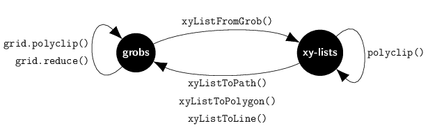
The grid.polyclip() function and the
grid.reduce() function accept 'grid' grobs
and return 'grid' grobs. This is the simplest user interface.
The xyListFromGrob() function converts a grob
into a list of xy-lists. It first converts a grob
to a "GridGrobCoords" (or "GridGTreeCoords") object using
grobCoords().
The "GridGrobCoords" (or "GridGTreeCoords") object is then
reduced to a list of xy-lists either by "flatten"ing all of the
"GridCoords" from the grob to a single list or by
combining shapes (one or more "GridCoords" from the same grob)
using polyclip::polyclip() and the operator specified
in reduceA or reduceB.
A gTree reduces each of its children and then combines the
reduced children together.
This function provides a to enter the 'polyclip'
world of lists of xy-lists, starting from a 'grid' grob.
The functions xyListToPath(),
xyListtoPolygon(), and
xyListToLine() convert back from a list of xy-lists to a grob.
There may be more than one xy-list, in which case,
xyListToPolygon() creates a grob that draws a
separate polygon for each xy-list,
xyListToPath() creates a grob that draws a single
path (using rule to determine the interior of the path),
and xyListToLine() creates a grob that draws a separate line
for each xy-list.
These functions allow the user to return from the 'polyclip'
world back to the world of 'grid' grobs.
The polyclip() function takes
a list of xy-lists and returns a list of xy-lists.
This allows the user to perform calculations in the 'polyclip'
world. For example, we can use xyListFromGrob() to
generate coordinates from a closed 'grid'
grob, but then work with them as if they are coordinates from an
open shape.
When a list of xy-lists is fed to polyclip::polyclip(),
a fill rule is specified to determine the interior of the shape
that is described by the list of xy-lists.
When we convert a grob to a list of xy-lists, the fill rule may
be included in the grobCoords() result (e.g.,
if we are converting a path grob), but it may not.
The fill rule that gets sent to polyclip::polyclip()
is determined as follows: if the user specifies
fillA or fillB explicitly, that fill
rule is used; otherwise, if the grobCoords() result
contains a fill rule, that is used; otherwise the fill rule is
"nonzero" (the 'polyclip' way of saying "winding").
Note that this is different from the default of "evenodd" that
polyclip::polyclip() itself uses.
The grobCoords() function has a closed
argument to indicate whether we want the coordinates of a closed
shape or an open shape.
From R 4.3.0 or from 'gridGeometry' 0.3-1, where it can
be determined that the grob is open, closed defaults
to FALSE. Otherwise, closed defaults
to TRUE. Prior to that, the closed
argument must be specified explicitly.
When we ask for the coordinates from a polygon grob,
we get the coordinates of the polygon if closed=TRUE, but
we get nothing ("empty" coordinates) if closed=FALSE.
Similarly, if we ask for the coordinates from a line grob,
we get the coordinates of the line if closed=FALSE, but
we get nothing if closed=TRUE.
A gTree presents a problem because it can contain grobs that draw
both open and closed shapes.
The grid.polyclip() function handles this problem
by generating open coordinates for A
and combining them with B
and then also generating closed coordinates
for A
and combining them with B.
The final result is then a gTree that
combines the open result and the closed result.
The following code shows an example where A is a
gTree consisting of a line and a rectangle and B
is a circle grob (and the operator is "minus").
The result is a combination of the (closed)
rectangle minus the (closed) circle and the (open) line
minus the (closed) circle.
grid.polyclip(gTree(children=gList(rectGrob(width=.5, height=.5),
                                   segmentsGrob(0, .5, 1, .5))),
              circleGrob(r=.2),
              "minus",
              gp=gpar(fill="grey"))

Note that B cannot be open,
a limitation imposed by the underlying
Clipper library (Johnson, 2019).
On the other hand, the Clipper library does allow A
to be a combination of open and closed shapes
(though the semantics of that can be tortuous),
whereas 'gridGeometry' only ever calls polyclip::polyclip()
with either A entirely closed or
A entirely open.
By default, any grob (including gTrees) that draws more than one
shape will be reduced. When closed=TRUE, the
result will be a single shape based on the union of the multiple shapes.
The 'polyclip' package (and the Clipper
library) will accept a list of xy-lists, i.e., multiple shapes,
so should we always reduce multiple shapes to a single shape?
By default, we do always reduce, but the user has the option
of specifying op="flatten", which will result in
sending multiple shapes to 'polyclip'.
The main idea behind the changes to grobCoords is to provide more detailed and comprehensive information about the coordinates for a 'grid' grob. We want to retain information about where the sets of coordinates came from through both a hierarchical structure and labelling of components within that structure.
The 'gridGeometry' package makes some use of that extra information, e.g., to determine the fill rule that it sends to 'polyclip' functions.
The grobCoords() function is also
used by 'grid' itself for resolving fill patterns
(Murrell, 2022b),
by making use of the names on grobCoords() output.
In that case, the extra information is important because it allows
us to resolve a pattern relative to individual shapes within a grob
as well as relative to the bounding box around all shapes within a
grob.
It is also hoped that the extra information provided by
grobCoords() may prove useful to
code writers and package developers that make use of
grobCoords() output.
One speculative application is for graphics device packages
that do not natively support some of the new graphics engine
features, like affine transformations, to add support for some
features by
working with grob coordinates. For example, a transformed
circle could be produce by calculating the coordinates
of the original circle, transforming the coordinates, and drawing the
transformed coordinates as a polygon.
The examples and discussion in this report relate to R version 4.2.0 and 'gridGeometry' version 0.3-1.
This report was generated within a Docker container (see Resources section below).
Murrell, P. (2022). "Constructive Geometry for Complex Grobs" Technical Report 2022-02, Department of Statistics, The University of Auckland. Version 1. [ bib | DOI | http ]
This document
by Paul
Murrell is licensed under a Creative
Commons Attribution 4.0 International License.