 http://orcid.org/0000-0002-3224-8858
by Paul Murrell
 http://orcid.org/0000-0002-3224-8858
Version 4: Tuesday 14 April 2020
Version 1: original publication
Version 2: added mention of 'ggforce' and 'ggraph'
Version 3: Wednesday 01 May 2019; 'gridGeometry' now depends on 'polyclip' 1.10-0
Version 4: start adding dates to history

This document
by Paul
Murrell is licensed under a Creative
Commons Attribution 4.0 International License.
This report describes a new function in 'grid' called
grobCoords and a new package called 'gridGeometry'
that combines grobCoords with the 'polyclip'
package to provide a geometry engine interface for 'grid'.
The 'grid' package for R (R Core Team, 2018) provides some useful tools, such as units, viewports, and layouts, that make it easy to express certain arrangements of output when drawing (e.g., 'ggplot2' plots; Wickham, 2016). However, there are many graphical results that are difficult to produce with 'grid'. A simple example is drawing an edge between two nodes on a graph or diagram, as shown below.
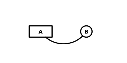
To be more specific, the line between the two nodes in the above
diagram is a Bezier curve that would originate and terminate at the centre
of the two nodes, if it were not cut off at the node boundaries.
This means that 'grid' functions like grobX and
grobY are no use, because it is difficult to
determine the angle of incidence of the lines to the nodes.
We could use grid.bezier, starting at the
boundaries of the nodes, but that would produce a different curve entirely,
and one that would not be aiming at the node centres.
Another detail about the diagram is that the background of the nodes is transparent (as shown below). This means that the standard R graphics "painters model" cannot help us out; we cannot just draw a Bezier curve that starts and ends at the node centres and then draw opaque nodes over the top to obscure the intersection of the curve with the nodes.
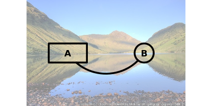
The photo in the image above is © Mick Garratt (Loch na Leitreach, Sunday, 7 June, 2009, cc-by-sa/2.0). It is read into R using the 'jpeg' package (Urbanek, 2014)
One way to produce the diagram above is using "constructive geometry", where we create a shape that is difficult to describe by combining shapes that are easier to describe. In the example above, the curve between the nodes is difficult to describe, but a curve between the node centres is easy and the nodes themselves are easy. By "subtracting" the nodes from a curve between the node centres we can easily obtain the curve between the nodes. This document describes a new package for R called 'gridGeometry' (Murrell, 2019) that provides tools for performing this sort of constructive geometry with 'grid' graphics.
library(gridGeometry)
The following code uses standard 'grid' functions to describe two nodes (a rectangle and a circle) at locations A and B and a Bezier curve from A to B.
Ax <- .3
Ay <- .5
Bx <- .7
By <- .5
node1 <- rectGrob(Ax, Ay, .2, .2,
                  gp=gpar(lwd=5, fill=NA))
node2 <- circleGrob(Bx, By, r=.1,
                    gp=gpar(lwd=5, fill=NA))
line <- bezierGrob(c(Ax, .4, .6, Bx),
                   c(Ay, .2, .2, By),
                   gp=gpar(col=rgb(0,0,0,.2), lwd=5))
The polyclipGrob function from the 'gridGeometry'
package can be used to create a new grob that is the Bezier
curve "minus" the two nodes.
p <- polyclipGrob(line, gList(node1, node2), op="minus",
                  gp=gpar(lwd=5))
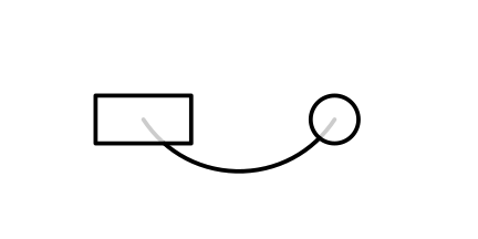
The diagram below shows the two nodes, the original Bezier curve (in grey), and the constructed Bezier curve (the grey curve minus the nodes).
The next section describes the 'gridGeometry' package in more detail and later sections provide some more examples of its use.
The 'gridGeometry' package provides functions for combining or transforming 'grid' grobs to create new grobs.
The grid.polyclip function, and the polyclipGrob
function, allow us to combine grobs using operations supported by the
polyclip function from the 'polyclip' package
(Johnson and Baddeley, 2019)
(which is an R interface to the C Clipper library; Johnson, 2019).
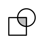
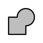
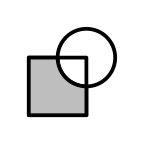
The following code demonstrates the four polyclip
operations: intersection, union, minus, and xor.
In each case, we combine an overlapping rectangle and circle
(both drawn with thick black outlines) and the result is drawn
as a filled grey shape with thick black outline.
r <- rectGrob(.4, .4, .4, .4, gp=gpar(lwd=5))
c <- circleGrob(.6, .6, r=.2, gp=gpar(lwd=5))
grid.draw(r)
grid.draw(c)
grid.polyclip(r, c, op="intersection",
              gp=gpar(lwd=5, fill="grey"))
grid.draw(r)
grid.draw(c)
grid.polyclip(r, c, op="union",
              gp=gpar(lwd=5, fill="grey"))
grid.draw(r)
grid.draw(c)
grid.polyclip(r, c, op="minus",
              gp=gpar(lwd=5, fill="grey"))
grid.draw(r)
grid.draw(c)
grid.polyclip(r, c, op="xor",
              gp=gpar(lwd=5, fill="grey"))

The 'gridGeometry' package is based on a fork
of the 'polyclip' package that allows these operations to
occur on (open) lines as well as (closed) polygons.
The following code demonstrates the four polyclip
operations when combining a Bezier curve with an overlapping circle.
In each case, the curve and the circle are drawn with a thin black
line and the result is drawn with a thick black line.
l <- bezierGrob(c(.2, .4, .6, .8),
                c(.2, .8, .8, .2))
c <- circleGrob(.6, .6, r=.2)
grid.draw(l)
grid.draw(c)
grid.polyclip(l, c, op="intersection",
              gp=gpar(lwd=5))

grid.draw(l)
grid.draw(c)
grid.polyclip(l, c, op="union",
              gp=gpar(lwd=5))

grid.draw(l)
grid.draw(c)
grid.polyclip(l, c, op="minus",
              gp=gpar(lwd=5))

grid.draw(l)
grid.draw(c)
grid.polyclip(l, c, op="xor",
              gp=gpar(lwd=5))

The other high-level functions in 'gridGeometry' are
grid.trim and trimGrob.
These allow us to extract subsets of a line by
specifying from and to
arguments. The following code demonstrates its use by
creating a variety of subsets of a Bezier curve.
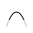
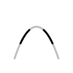
In each case, the complete curve is drawn as a thick grey line
and the subsets are drawn as thick black lines.
l <- bezierGrob(c(.2, .4, .6, .8),
                c(.2, .8, .8, .2),
                gp=gpar(col="grey", lwd=5))
The from and to arguments
specify proportions of the
length of the line. In the example below, we create a subset
that starts 20% of the way along the curve and finishes
80% of the way along the curve.
grid.draw(l)
grid.trim(l, .2, .8, gp=gpar(lwd=5))
Both from and to
can be vectors, in which case multiple subsets are created.
In the example below, we generate a subset from 20% to 40% and
another subset from 60% to 80% of the way along the curve.
grid.draw(l)
grid.trim(l, c(.2, .6), c(.4, .8), gp=gpar(lwd=5))
Both from and to
can also be negative, in which case the
distance is measured from the end of the line.
In the example below, we create a subset that starts 20% of the
way along the curve and finishes 10% from the end of the curve.
grid.draw(l)
grid.trim(l, .2, -.1, gp=gpar(lwd=5))
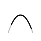
Both from and to
can be 'grid' units. In the example below, we create a subset
that starts 5mm along the curve and finishes 1in from the end
of the curve.
grid.draw(l)
grid.trim(l, unit(5, "mm"), unit(-1, "in"), gp=gpar(lwd=5))
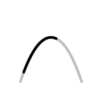
When from and to are units,
the "npc" coordinate system represents 0 to 1 along the line.
This allows distances along the line to be specified
as a combination of a proportions and units.
In the example below, we create a subset that starts 20% of the
way along the curve and finishes 5mm past 50% of the way
along the curve.
grid.draw(l)
grid.trim(l, .2, unit(.5, "npc") + unit(5, "mm"), gp=gpar(lwd=5))
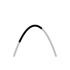
There is also a rep argument that can be used to repeat
from and to until the end of the
line. The values are repeated by adding the from
and to values onto the largest to value.
In other words, the line that remains after the last
to value is then used to generate more subsets using the
original from and to values, and that process is
repeated until there is no line left.
In the example below, we create a subset
that starts at 10% and finishes at 20%, then we create a subset
that starts at 30% and finishes at 40%, and so on until a final
subset that starts at 90% and finishes at 100%.
grid.draw(l)
grid.trim(l, .1, .2, rep=TRUE, gp=gpar(lwd=5))
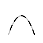
The high-level functions like
grid.polyclip begin with 'grid' grobs
and generate 'grid' grobs as the result (and draw them).
In between, they have to convert 'grid' grobs
into a set of coordinates that can be fed to
polyclip from the 'polyclip' package
and then convert the result from polyclip
back to a 'grid' grob. This section and the next section
look at some functions that allow us to perform these
conversions directly. This is useful if we want
more control over the conversions between grobs and coordinates
and if we want to perform further transformations on coordinates
before converting back to grobs.
The conversion from a grob to a set of coordinates
is made possible by the new function grobCoords
in the 'grid' package. This
function converts a grob into a list containing lists of x/y coordinates,
with all values in inches relative to the current 'grid' viewport.
There is also a closed argument to indicate whether
we are looking for the coordinates of a closed shape or an open shape.
This is straightforward for something like a single line.
In the example below, we have a grob that specifies a line from
the point (2in, 2in) to (3in, 3in) within the current viewport.
Converting that to a set of coordinates in inches within the
current viewport produces the expected result.
l <- linesGrob(unit(2:3, "in"), unit(2:3, "in"))
lcoords <- grobCoords(l, closed=FALSE)
lcoords
  [[1]]
  [[1]]$x
  [1] 2 3

  [[1]]$y
  [1] 2 3
However, some grobs generate many more coordinates.
For example, in the case of a circle, the grob contains
only centre and radius information, but the grob coordinates
is a list of explicit points on the circumference of the circle.
In the example below, we describe a circle centred at (2in, 2in)
with a radius of 1in. The set of coordinates in inches within the
current viewport consists of 100 (x, y) locations.
(There is a argument n to control how many
coordinates are generated for a circle).
c <- circleGrob(2, 2, 1, default.units="in")
ccoords <- grobCoords(c, closed=TRUE)
ccoords
  [[1]]
  [[1]]$x
    [1] 3.000000 2.998027 2.992115 2.982287 2.968583 2.951057 2.929776 2.904827 2.876307 2.844328
   [11] 2.809017 2.770513 2.728969 2.684547 2.637424 2.587785 2.535827 2.481754 2.425779 2.368125
   [21] 2.309017 2.248690 2.187381 2.125333 2.062791 2.000000 1.937209 1.874667 1.812619 1.751310
   [31] 1.690983 1.631875 1.574221 1.518246 1.464173 1.412215 1.362576 1.315453 1.271031 1.229487
   [41] 1.190983 1.155672 1.123693 1.095173 1.070224 1.048943 1.031417 1.017713 1.007885 1.001973
   [51] 1.000000 1.001973 1.007885 1.017713 1.031417 1.048943 1.070224 1.095173 1.123693 1.155672
   [61] 1.190983 1.229487 1.271031 1.315453 1.362576 1.412215 1.464173 1.518246 1.574221 1.631875
   [71] 1.690983 1.751310 1.812619 1.874667 1.937209 2.000000 2.062791 2.125333 2.187381 2.248690
   [81] 2.309017 2.368125 2.425779 2.481754 2.535827 2.587785 2.637424 2.684547 2.728969 2.770513
   [91] 2.809017 2.844328 2.876307 2.904827 2.929776 2.951057 2.968583 2.982287 2.992115 2.998027

  [[1]]$y
    [1] 2.000000 2.062791 2.125333 2.187381 2.248690 2.309017 2.368125 2.425779 2.481754 2.535827
   [11] 2.587785 2.637424 2.684547 2.728969 2.770513 2.809017 2.844328 2.876307 2.904827 2.929776
   [21] 2.951057 2.968583 2.982287 2.992115 2.998027 3.000000 2.998027 2.992115 2.982287 2.968583
   [31] 2.951057 2.929776 2.904827 2.876307 2.844328 2.809017 2.770513 2.728969 2.684547 2.637424
   [41] 2.587785 2.535827 2.481754 2.425779 2.368125 2.309017 2.248690 2.187381 2.125333 2.062791
   [51] 2.000000 1.937209 1.874667 1.812619 1.751310 1.690983 1.631875 1.574221 1.518246 1.464173
   [61] 1.412215 1.362576 1.315453 1.271031 1.229487 1.190983 1.155672 1.123693 1.095173 1.070224
   [71] 1.048943 1.031417 1.017713 1.007885 1.001973 1.000000 1.001973 1.007885 1.017713 1.031417
   [81] 1.048943 1.070224 1.095173 1.123693 1.155672 1.190983 1.229487 1.271031 1.315453 1.362576
   [91] 1.412215 1.464173 1.518246 1.574221 1.631875 1.690983 1.751310 1.812619 1.874667 1.937209
It is also possible for a single 'grid' grob to describe
several shapes. In this case, the set of coordinates is a list
with more than one component. In the example below,
the grob describes two straight lines, one from (1in, 1in)
to (2in, 2in) and one from (3in, 3in) to (4in, 4in).
The result from grobCoords is a list of two
sets of (x, y) coordinates.
p <- polylineGrob(1:4, 1:4, default.units="in", id=rep(1:2, each=2))
grobCoords(p, closed=FALSE)
  $`1`
    x y
  1 1 1
  2 2 2

  $`2`
    x y
  3 3 3
  4 4 4
If we ask an open shape for closed coordinates, or a closed shape for open coordinates, we get an empty result. In the example below, we are asking an (open) line segment for closed coordinates.
grobCoords(l, closed=TRUE)
  $x
  [1] 0

  $y
  [1] 0
isEmptyCoords(grobCoords(l, closed=TRUE))
[1] TRUE
The reason for distinguishing between open and closed coordinates is because it is possible to create a 'grid' grob that consists of both open and closed components. In the example below, we create a gTree grob that has an (open) line and a (closed) circle as its children. When we ask this gTree for closed coordinates, we get an empty result from the line, but a full set of coordinates from the circle.
gt <- gTree(children=gList(l, c))
grobCoords(gt, closed=TRUE)
  $GRID.lines.34
  $GRID.lines.34$x
  [1] 0

  $GRID.lines.34$y
  [1] 0


  $GRID.circle.35
  $GRID.circle.35$x
    [1] 3.000000 2.998027 2.992115 2.982287 2.968583 2.951057 2.929776 2.904827 2.876307 2.844328
   [11] 2.809017 2.770513 2.728969 2.684547 2.637424 2.587785 2.535827 2.481754 2.425779 2.368125
   [21] 2.309017 2.248690 2.187381 2.125333 2.062791 2.000000 1.937209 1.874667 1.812619 1.751310
   [31] 1.690983 1.631875 1.574221 1.518246 1.464173 1.412215 1.362576 1.315453 1.271031 1.229487
   [41] 1.190983 1.155672 1.123693 1.095173 1.070224 1.048943 1.031417 1.017713 1.007885 1.001973
   [51] 1.000000 1.001973 1.007885 1.017713 1.031417 1.048943 1.070224 1.095173 1.123693 1.155672
   [61] 1.190983 1.229487 1.271031 1.315453 1.362576 1.412215 1.464173 1.518246 1.574221 1.631875
   [71] 1.690983 1.751310 1.812619 1.874667 1.937209 2.000000 2.062791 2.125333 2.187381 2.248690
   [81] 2.309017 2.368125 2.425779 2.481754 2.535827 2.587785 2.637424 2.684547 2.728969 2.770513
   [91] 2.809017 2.844328 2.876307 2.904827 2.929776 2.951057 2.968583 2.982287 2.992115 2.998027

  $GRID.circle.35$y
    [1] 2.000000 2.062791 2.125333 2.187381 2.248690 2.309017 2.368125 2.425779 2.481754 2.535827
   [11] 2.587785 2.637424 2.684547 2.728969 2.770513 2.809017 2.844328 2.876307 2.904827 2.929776
   [21] 2.951057 2.968583 2.982287 2.992115 2.998027 3.000000 2.998027 2.992115 2.982287 2.968583
   [31] 2.951057 2.929776 2.904827 2.876307 2.844328 2.809017 2.770513 2.728969 2.684547 2.637424
   [41] 2.587785 2.535827 2.481754 2.425779 2.368125 2.309017 2.248690 2.187381 2.125333 2.062791
   [51] 2.000000 1.937209 1.874667 1.812619 1.751310 1.690983 1.631875 1.574221 1.518246 1.464173
   [61] 1.412215 1.362576 1.315453 1.271031 1.229487 1.190983 1.155672 1.123693 1.095173 1.070224
   [71] 1.048943 1.031417 1.017713 1.007885 1.001973 1.000000 1.001973 1.007885 1.017713 1.031417
   [81] 1.048943 1.070224 1.095173 1.123693 1.155672 1.190983 1.229487 1.271031 1.315453 1.362576
   [91] 1.412215 1.464173 1.518246 1.574221 1.631875 1.690983 1.751310 1.812619 1.874667 1.937209
If we ask the gTree for open coordinates, we get coordinates from the line and an empty result from the circle.
grobCoords(gt, closed=FALSE)
  $GRID.lines.34
  $GRID.lines.34$x
  [1] 2 3

  $GRID.lines.34$y
  [1] 2 3


  $GRID.circle.35
  $GRID.circle.35$x
  [1] 0

  $GRID.circle.35$y
  [1] 0
Once we have grob coordinates, we can call functions like
polyclip from the 'polyclip' package to
combine the coordinates. The result is a new set of coordinates.
In the example below, we intersect the line with the circle and the result
is a truncated line (up to the edge of the circle).
The closed argument (which has been added in the
fork of the 'polyclip' package) tells polyclip whether
its first argument is open or closed (polyclip
requires the second argument to always be a closed shape).
polyclip(lcoords, ccoords, closed=FALSE)
  [[1]]
  [[1]]$x
  [1] 2.000000 2.706758

  [[1]]$y
  [1] 2.000000 2.706758
We can also use a set of coordinates in other calculations.
For example, the following code draws a variable-width line
around the circumference of the circle (using the 'vwline'
package; , Murrell, 2018).
The value of grobCoords here is to convert
a circle specification into (essentially)
a series of straight line segments,
which we can then use with the grid.vwcurve
function to draw a variable-width line.
library(vwline)
cx <- ccoords[[1]]$x
cy <- ccoords[[1]]$y
grid.vwcurve(cx, cy, default.units="in",
             w=seq(0, 1, length.out=length(cx)))

The 'gridGeometry' package also defines a generic version
of the polyclip function, with
polyclip::polyclip as the default and a
new method for 'grid' grobs. This means that
we can generate coordinates for a combination of grobs directly.
The following code sends polyclip the original
grobs rather than their coordinates. The result is still
a set of coordinates.
polyclip(l, c, closed=FALSE)
  [[1]]
  [[1]]$x
  [1] 2.000000 2.706758

  [[1]]$y
  [1] 2.000000 2.706758
There is also a polyclip method for gPaths, so that
it is possible to refer by name to grobs that have already been drawn.
The following code demonstrates this by drawing a line named
"l" and a circle named "c"
and then calling polyclip to produce coordinates for the
intersection of the grobs named "l" and "c".
grid.lines(unit(2:3, "in"), unit(2:3, "in"), name="l")
grid.circle(2, 2, 1, default.units="in", name="c")
polyclip("l", "c", closed=FALSE)
  [[1]]
  [[1]]$x
  [1] 2.000000 2.706758

  [[1]]$y
  [1] 2.000000 2.706758
There is also a low-level function that underlies the
grid.trim and
trimGrob functions. The trim function
takes either a grob, or a set of coordinates, and
generates a new set of coordinates, in this case representing
one or more subsets of the original grob coordinates.
For example, in the code below, we generate an X-spline grob that
starts at (0in, 0in), ends at (2in, 01in) and passes through
(1in, 1in) and then we
call trim to calculate the coordinates of two
subsets of the X-spline curve: the first half of the curve
and the last half of the curve.
xg <- xsplineGrob(0:2, c(0, 1, 0), default.units="in", shape=-1)
xcoords <- trim(xg, from=0:1/2, to=1:2/2)
xcoords
  [[1]]
  [[1]]$x
   [1] 0.000 0.000 0.003 0.010 0.023 0.043 0.070 0.103 0.142 0.186 0.235 0.287 0.342 0.401 0.463 0.529
  [17] 0.600 0.676 0.759 0.848 0.942 1.000

  [[1]]$y
   [1] 0.000 0.001 0.006 0.020 0.045 0.082 0.132 0.192 0.260 0.335 0.414 0.493 0.572 0.648 0.720 0.787
  [17] 0.848 0.901 0.945 0.978 0.997 1.000


  [[2]]
  [[2]]$x
   [1] 1.000 1.000 1.096 1.189 1.275 1.355 1.429 1.498 1.562 1.623 1.680 1.734 1.785 1.832 1.875 1.911
  [17] 1.942 1.966 1.983 1.993 1.998 2.000 2.000

  [[2]]$y
   [1] 1.000 1.000 0.991 0.966 0.929 0.881 0.824 0.761 0.692 0.618 0.541 0.461 0.382 0.305 0.232 0.166
  [17] 0.110 0.066 0.034 0.014 0.003 0.000 0.000
The following code draws the two halves of the curve with different line widths.
pushViewport(viewport(width=2/3, height=2/3))
grid.lines(xcoords[[1]]$x, xcoords[[1]]$y, default.units="in",
           gp=gpar(lwd=3, lineend="butt"))
grid.lines(xcoords[[2]]$x, xcoords[[2]]$y, default.units="in",
           gp=gpar(lwd=10, lineend="butt"))
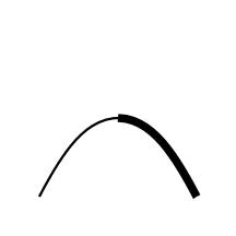
If we have worked directly in the world of grob coordinates, using functions from the previous section, we usually want to get back to the world of grobs, so that we can draw the final result.
We have seen a couple of examples of drawing shapes from
coordinates by calling 'grid' functions and taking into
account that the coordinates in are inches.
The 'gridGeometry' package provides several convenience functions
that make this job a little less work:
xyListLine, xyListPath and
xyListPolygon.
The main benefit of these functions is that they automatically
assume inches as the coordinate system and they automatically
handle multiple shapes. For example, in the following code
we subtract a
thin rectangle from a circle using polyclip
directly, so the result is a set of coordinates.
coords <- polyclip(c, rectGrob(width=.2), op="minus")
coords
  [[1]]
  [[1]]$x
   [1] 1.600000 1.574221 1.518246 1.464173 1.412215 1.362576 1.315453 1.271031 1.229487 1.190983
  [11] 1.155672 1.123693 1.095173 1.070224 1.048943 1.031417 1.017713 1.007885 1.001973 1.000000
  [21] 1.001973 1.007885 1.017713 1.031417 1.048943 1.070224 1.095173 1.123693 1.155672 1.190983
  [31] 1.229487 1.271031 1.315453 1.362576 1.412215 1.464173 1.518246 1.574221 1.600000

  [[1]]$y
   [1] 2.915983 2.904827 2.876307 2.844328 2.809017 2.770513 2.728969 2.684547 2.637424 2.587785
  [11] 2.535827 2.481754 2.425779 2.368125 2.309017 2.248690 2.187381 2.125333 2.062791 2.000000
  [21] 1.937209 1.874667 1.812619 1.751310 1.690983 1.631875 1.574221 1.518246 1.464173 1.412215
  [31] 1.362576 1.315453 1.271031 1.229487 1.190983 1.155672 1.123693 1.095173 1.084017


  [[2]]
  [[2]]$x
   [1] 2.425779 2.481754 2.535827 2.587785 2.637424 2.684547 2.728969 2.770513 2.809017 2.844328
  [11] 2.876307 2.904827 2.929776 2.951057 2.968583 2.982287 2.992115 2.998027 3.000000 2.998027
  [21] 2.992115 2.982287 2.968583 2.951057 2.929776 2.904827 2.876307 2.844328 2.809017 2.770513
  [31] 2.728969 2.684547 2.637424 2.587785 2.535827 2.481754 2.425779 2.400000 2.400000

  [[2]]$y
   [1] 1.095173 1.123693 1.155672 1.190983 1.229487 1.271031 1.315453 1.362576 1.412215 1.464173
  [11] 1.518246 1.574221 1.631875 1.690983 1.751310 1.812619 1.874667 1.937209 2.000000 2.062791
  [21] 2.125333 2.187381 2.248690 2.309017 2.368125 2.425779 2.481754 2.535827 2.587785 2.637424
  [31] 2.684547 2.728969 2.770513 2.809017 2.844328 2.876307 2.904827 2.915983 1.084017
The xyListPolygon function
automatically copes with the fact that the result is
two separate shapes and generates a polygon grob that we can draw.
grid.draw(xyListPolygon(coords,
                        gp=gpar(lwd=5, fill="grey")))
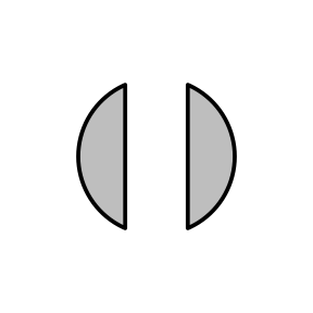
It is important to note that a call to the grobCoords
function is when grob coordinates get converted to inches
within the current 'grid' viewport. This means that the coordinates
that are generated are relative to the viewport in effect
when grobCoords is called.
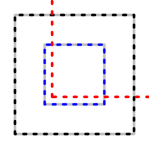
In the code below, we generate a rectangle grob and call
grobCoords to calculate its coordinates.
We then draw the rectangle grob and a polygon based on
its coordinates, in the same viewport that was in effect
when we calculated the coordinates, so the rectangle (grey)
and the polygon (dotted black) match up.
r <- rectGrob(width=.8, height=.8, gp=gpar(lwd=5, col="grey"))
coords <- grobCoords(r, closed=TRUE)
grid.draw(r)
grid.draw(xyListPolygon(coords,
                        gp=gpar(lwd=5, lty="dotted")))
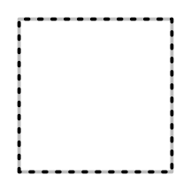
Next, we push a viewport (in the central quarter of the image) and draw the grob and the polygon within this viewport. This is not the viewport that the coordinates were calculated within, so the polygon (red dotted) does not match the rectangle (inner grey).
pushViewport(viewport(width=.5, height=.5))
grid.draw(r)
grid.draw(xyListPolygon(coords,
                        gp=gpar(lwd=5, lty="dotted", col="red")))
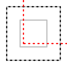
Finally, we call grobCoords again, this time within
the new viewport, and now the rectangle (inner grey) and the
polygon (dotted blue) match up again.
grid.draw(xyListPolygon(grobCoords(r, closed=TRUE),
                        gp=gpar(lwd=5, lty="dotted", col="blue")))
On the other hand, the grobCoords function automatically
takes into account any vp setting (and for gTrees any
childrenvp settings).
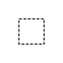
For example, in the following code we create a rectangle grob
with a vp argument that means that the rectangle
will be drawn in the central quarter of the image.
If we draw the rectangle (grey) and call grobCoords
and draw a polygon from the resulting coordinates (dotted black)
in the same viewport, we get a matching result.
r <- rectGrob(width=.8, height=.8,
              gp=gpar(lwd=5, col="grey"),
              vp=viewport(width=.5, height=.5))
grid.draw(r)
grid.draw(xyListPolygon(grobCoords(r, closed=TRUE),
                        gp=gpar(lwd=5, lty="dotted")))
It is also important to note that the coordinates generated by
grobCoords are "neutral" in the sense that they
do not retain any information about whether they were generated
from a closed or open shape, or any details like fill rules for
more complex shapes. This means that we can impose
semantics on the coordinates that are different from the
semantics of the original grob. As an example, consider the
following lines grob.
lg <- linesGrob(c(.2, .2, .8, .8, .4, .6),
                c(.2, .8, .8, .2, .6, .6),
                gp=gpar(lwd=3))
grid.draw(lg)
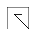
We can generate coordinates from this line and then
a grob from the coordinates and get a filled shape.
We must specify closed=FALSE for the call to
grobCoords
or we will get an empty result, but once we have coordinates
we can use them however we wish. In this case, by passing
the coordinates to the xyListPath function, we treat
the coordinates as a closed path shape.
lgcoords <- grobCoords(lg, closed=FALSE)
lgpath <- xyListPath(lgcoords, rule="evenodd", gp=gpar(fill="black"))
grid.draw(lgpath)

It is also possible
to dictate how coordinates are interpreted
when we call the polyclip function.
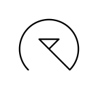
The following code treats the line coordinates as a closed shape
to intersect those coordinates with the coordinates for a circle.
We specify closed=TRUE in the call to
polyclip so that it interprets the coordinates
for the line as a closed shape.
coords <- polyclip(lgcoords,
                   grobCoords(circleGrob(.5, .5, .3), closed=TRUE),
                   closed=TRUE,
                   fillA="evenodd")
The result of polyclip is a new set of coordinates
and we can use them to draw an open line ...
grid.draw(xyListLine(coords, gp=gpar(lwd=3)))
... or a closed path ...
grid.draw(xyListPath(coords, gp=gpar(fill="black")))

This section looks at some important differences between 'grid' grobs and sets of coordinates.
The grobCoords function generates points on the
boundary of a 'grid' grob based on the basic description of the
shape of the grob.
This does not take into account things like
the colour of the grob, whether the grob is filled in or not,
or, more importantly, the thickness of the line used to draw
the boundary of the grob.
The following code demonstrates this difference by subtracting a rectangle from a circle, both of which are drawn with thick lines. The resulting intersection is drawn as a thin red line. Notice that only the basic circle shape has been subtracted from the rectangle, ignoring the thickness of the circle border and ignoring the thickness of the rectangle border.
r <- rectGrob(.4, .4, .4, .4, gp=gpar(lwd=10))
c <- circleGrob(.6, .6, r=.2, gp=gpar(lwd=10))
grid.draw(r)
grid.draw(c)
grid.polyclip(r, c, op="minus",
              gp=gpar(col="red"))

If we draw the result with the same line thickness as the circle and the rectangle, the result looks even worse (it looks like only the interior of the circle has been removed from the rectangle) ...
grid.draw(r)
grid.draw(c)
grid.polyclip(r, c, op="minus",
              gp=gpar(col="red", lwd=10))

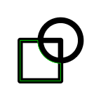
If we actually want to subtract the outline of the drawn border of the circle, we need coordinates that describe that outline. One way to do that is with the 'vwline' package, which generates a polygon or path to represent a line (potentially with a variable width).
The following code calls grobCoords to
get the coordinates of the rectangle and the circle. We then generate
a variable-width line (with a constant width) based on the circle
coordinates. Next, we generate the coordinates for that variable-width
line (which has coordinates for both the inside and outside of the
circle border). Finally, we generate a polygon by subtracting the
second set of coordinates for the variable-width line from
the rectangle coordinates.
rc <- grobCoords(r, closed=TRUE)
cc <- grobCoords(c, closed=TRUE)[[1]]
vwc <- vwcurveGrob(cc$x, cc$y, default.units="in", w=unit(10/96, "in"),
                   open=FALSE)
vwcc <- grobCoords(vwc, closed=TRUE)
result <- xyListPolygon(polyclip(rc, vwcc[2], "minus"), gp=gpar(col="green"))
The figure below shows the original rectangle, the variable-width line and result of the subtraction (in green). Many other variations on this result are possible by playing directly with coordinates of grobs.
grid.draw(r)
grid.draw(vwc)
grid.draw(result)
One simple application of 'gridGeometry' is to generate a polygonal shape that is difficult to describe directly, as in the original line between two graph nodes at the start of this document.
The code below shows a closed-shape version of this sort of task (for a fairly arbitrary shape). The goal is a rectangle with circular holes punched in it, including semicircular holes at the edges (the filled grey region below). This shape could be described explicitly as a path in 'grid', but it is much easier to describe a rectangle and a series of circles and subtract the latter from the former.
r <- rectGrob(width=.6, height=.4, gp=gpar(lwd=5))
c <- circleGrob(x=1:4/5, r=unit(5, "mm"), gp=gpar(lwd=5))
p <- polyclipGrob(r, c, op="minus",
                  gp=gpar(fill=rgb(0,0,0,.5), lwd=5))
grid.draw(r)
grid.draw(c)
grid.draw(p)

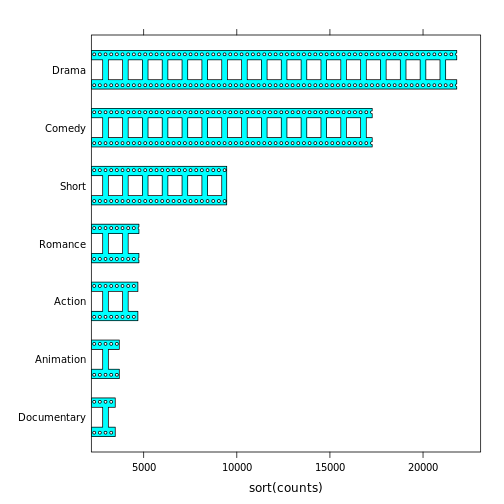
The next example shows a similar construction, but in a larger context
(at the risk of inviting the attention of the chart-junk police).
The overall plot is a 'lattice' barchart (Sarkar, 2008)
of counts of movies
in different genres (Wickham, 2015).
We have provided a panel function
that, after drawing the normal bars,
constructs a
"flim strip" shape by substracting lots of small rectangles and circles
from the normal bars.
This demonstrates the use of a gPath as the first argument
to grid.polyclip which, by default,
replaces the named grob with the result of the polyclip
operation (by default
retaining the graphical parameters of the original grob).
library(ggplot2movies)
counts <- apply(movies[-(1:17)], 2, sum)
filmstrip <- function(x, y, box.width=2/3, ...) {
    panel.barchart(x, y, box.width, ...)
    w <- convertWidth(unit(1, "npc"), "cm", valueOnly=TRUE)
    hsteps <- seq(-.1, w, .7)
    hx <- rep(hsteps, length(x))
    hy <- rep(y, each=length(hsteps))
    holes <- rectGrob(x=unit(hx, "cm"), y=unit(hy, "native"),
                      width=unit(.5, "cm"), height=unit(.7, "cm"),
                      just="left")
    esteps <- seq(.1, w, .2)
    ex <- rep(esteps, 2*length(x))
    ey <- rep(c(as.numeric(y) + .4*box.width,
                as.numeric(y) - .4*box.width),
              each=length(esteps))
    edges <- circleGrob(unit(ex, "cm"), unit(ey, "native"),
                        r=unit(.5, "mm"))
    grid.polyclip("plot_01.barchart.rect.panel.1.1",
                  gList(holes, edges), "minus")
}
library(lattice)
barchart(sort(counts),
         panel=function(x, y, ...) {
             filmstrip(x, y, ...)
         })
The next example demonstrates an application of the trim
function. To motivate the problem, we first draw a Bezier curve
with an arrow head with standard 'grid' functions.
x <- c(.2, .5, .5, .8)
y <- c(.2, 0, 1, .8)
grid.bezier(x, y, gp=gpar(lwd=5, fill=NA),
            arrow=arrow(angle=20, length=unit(1, "cm"), type="closed"))

There are two problems with the result above: the arrow head is drawn with the same graphical parameters as the line, so it is thick with rounded corners; and the orientation of the arrow head is based on the angle of the last straight line segment in the "curve", so it looks silly (because the end of the line has high curvature).
We are going to improve the arrow head by drawing the curve in separate parts. First, we get the coordinates for the line and split those into three parts: the last 10mm of the curve; 8mm from the end to 12mm from the end of the curve; and all but the last 10mm of the curve.
bg <- bezierGrob(x, y, gp=gpar(lwd=5, col=rgb(0,0,0,.2)))
pts <- grobCoords(bg, closed=FALSE)
segs <- trim(pts,
             from=unit(c(1, -8, -10), c("npc", "mm", "mm")),
             to=unit(c(-10, -12, 0), c("mm", "mm", "npc")))
Now we can draw most of the curve as a normal line and then add a variable-width line based on the last 10mm of the curve to produce an arrow head that follows the curve.
line <- xyListLine(segs[3], gp=gpar(lwd=5))
arrow <- offsetXsplineGrob(segs[[1]]$x, segs[[1]]$y, default.units="in",
                           shape=1,
                           w=widthSpline(unit(c(6, 0), "mm")))
grid.draw(line)
grid.draw(arrow)
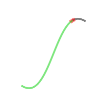
The following code takes this a step further and adds in a bit of constructive geometry. This time we draw all but the last 8mm of the curve as a normal line. We then create two variable-width lines, one based on the last 10mm of the curve as before, and a second based on the section of the curve from 8mm to 12mm from the end. We make the latter variable-width line expand much faster than the former (the two variable-width lines are shown in semitransparent red and semitransparent blue below).
line <- xyListLine(segs[2:3], gp=gpar(lwd=5))
arrow1 <- offsetXsplineGrob(segs[[1]]$x, segs[[1]]$y, default.units="in",
                            shape=1,
                            w=widthSpline(unit(c(6, 0), "mm")),
                            gp=gpar(fill=rgb(1,0,0,.5)))
arrow2 <- offsetXsplineGrob(segs[[2]]$x, segs[[2]]$y, default.units="in",
                            shape=1,
                            w=widthSpline(unit(c(12, 0), "mm")),
                            gp=gpar(fill=rgb(0,0,1,.5)))
grid.draw(line)
grid.draw(arrow1)
grid.draw(arrow2)
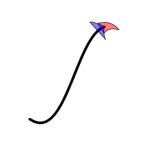
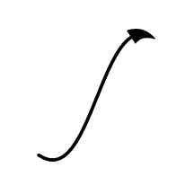
We construct a final arrow head by subtracting one variable-width line from the other to produce a curve with a notched arrow head that follows the curve (and has nice pointy corners).
arrow <- polyclipGrob(arrow1, arrow2, "minus",
                      gp=gpar(fill="black"))
grid.draw(line)
grid.draw(arrow)
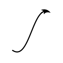
That may seem like a lot of work, but because it is code-based, this approach could easily be wrapped into a function to simplify reuse and enhance generality.
This report has described two new graphics facilities in R.
One is the grobCoords function in the 'grid'
package, which can be used to convert 'grid' grobs into
sets of coordinates that describe the shape of the grob.
The other is the 'gridGeometry' package, which provides
functions for combining grobs, for example, calculating the intersection
of two grobs.
It might reasonably be asked what purpose the 'gridGeometry' package is
really serving. The grobCoords function performs the
conversion from grobs into coordinates and the
'polyclip' package does all of the hard work of
combining sets of coordinates. What does 'gridGeometry' add to that?
The answer is, mostly, just convenience. Most of the functions
in the 'gridGeometry' package are there to provide an interface
to the process of combining 'grid' grobs.
However, the grid.trim function for
generating subsets of lines is also a new contribution.
What is the value of having this convenient interface to a geometry engine? The main idea is that this provides access to a new tool. For example, prior to having this tool, we might never have thought of turning a bar plot into a film strip. Some might argue that we should never have that thought and that that is not a good thought, but the important point is that new tools help us to think of new ways of doing things. New tools help us to find new solutions to problems.
There are several other R packages that make use of
the geometry engine that is provided by the
'polyclip' package.
For example, 'eulerr' (Larsson, 2019) and
'SubgrPlots' (Ballarini and Chiu, 2018) use 'polyclip'
for drawing (variations
of) venn diagrams. The 'maptools' package (Bivand and Lewin-Koh, 2019)
uses 'polyclip'
to clip map regions (when they
wrap from left-edge to right-edge of map, or vice versa) and 'deldir'
(Turner, 2019)
uses 'polyclip' for complex clipping of voronoi tesselations.
The 'ggforce' (Pedersen, 2019) and
'ggraph' (Pedersen, 2018)
packages use 'polyclip' for
tasks very similar to those
demonstrated in this report (cutting edges between nodes and
modifying or combining shapes), but provides these facilities
as 'ggplot2' extensions rather than at the level of 'grid'.
The 'spatstat' package (Baddeley et al., 2015) uses 'polyclip'
for all sorts of things, including polygon offsets, polyline offsets, and
polygon intersection. The main difference betweeen 'gridGeometry'
and these other packages is in how the shapes that are to be combined
are generated.
The contribution of 'gridGeometry' (and grid::grobCoords)
is to add the ability to generate shapes
from 'grid' grobs (which includes anything that is drawn by
packages that are built on top of 'grid').
The usual issue of speed (or slowness) is a problem for the 'gridGeometry' package. This is not the fastest possible way to perform constructive geometry. However, in some applications and for some users, the convenience may be worth the wait.
Another important limitation of 'gridGeometry', or more specifically,
the grobCoords function, is that it is not
(currently) possible
to generate a set of coordinates for all 'grid' grobs.
It is perhaps not surprising that raster grobs, "clip" grobs, and
"null" grobs generate an empty set of coordinates, but,
in addition, text grobs and point grobs generate an empty set of
coordinates. These gaps may be the subject of future work.
The examples and discussion in this document relate to version
0.2-0 of the 'gridGeometry' package, version 1.10-0 of the
'polyclip' package (to allow for open paths), and R version 3.6.0
(for the grobCoords function).
This report was generated within a Docker container (see Resources section below).
Murrell, P. (2019). "A Geometry Engine Interface for 'grid'" Technical Report 2019-01, Department of Statistics, The University of Auckland. Version 4. [ bib | DOI | http ]

This document
by Paul
Murrell is licensed under a Creative
Commons Attribution 4.0 International License.