 http://orcid.org/0000-0002-3224-8858
by Jack Wong and Paul Murrell
http://orcid.org/0000-0002-3224-8858
Version 1: Wednesday 14 December 2022

This document
by Jack Wong and Paul
Murrell is licensed under a Creative
Commons Attribution 4.0 International License.
This document describes new functions in the 'gridGeometry' package for R that generate offset regions and Minkowski Sums for lines and polygons.
The 'gridGeometry' package
(Murrell, 2019;
Murrell, 2022a)
provides a 'grid' interface to
the polyclip() function from the 'polyclip' package
(Johnson and Baddeley, 2019).
This means that we can generate and draw a complex shape in 'grid'
by combining simple 'grid' shapes.
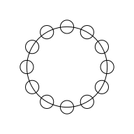
For example, the following code
defines a collection of simple circles:
a large circle and several smaller circles
that are arranged around the boundary of the large circle.
library(grid)
t <- seq(0, 2*pi, length.out=13)[-1]
x <- .5 + .3*cos(t)
y <- .5 + .3*sin(t)
bigC <- circleGrob(r=.3, gp=gpar(fill=NA))
littleC <- circleGrob(x, y, r=.05, gp=gpar(fill=NA))
grid.draw(bigC)
grid.draw(littleC)
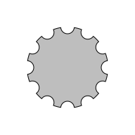
The next code generates a more complex "gear" shape by
subtracting the smaller circles from the large circle
using the grid.polyclip() function from the
'gridGeometry' package.
library(gridGeometry)
grid.polyclip(bigC, littleC, "minus",
              gp=gpar(fill="grey"))
This report describes an extension of the 'gridGeometry' package
to provide interfaces to three other functions from the 'polyclip'
package: polyoffset(), polylineoffset(),
and polyminkowski().
Two main functions have been added to 'gridGeometry'
for drawing offset regions: grid.polyoffset() and
grid.polylineoffset().
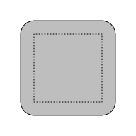
The grid.polyoffset() function takes a closed shape,
such as a rectangle or circle, and generates an offset region
based on a fixed offset given by
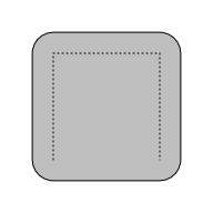
delta. For example, the following code
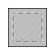
defines a rectangle and then draws an offset region based on
that rectangle with an offset of 5mm. The original rectangle
is shown as a dotted outline.
r <- rectGrob(width=.5, height=.5, gp=gpar(lty="dotted", fill=NA))
grid.polyoffset(r, unit(5, "mm"), gp=gpar(fill="grey"))
grid.draw(r)
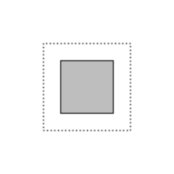
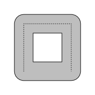
The offset can also be negative, as shown in the following code.
grid.polyoffset(r, unit(-5, "mm"), gp=gpar(fill="grey"))
grid.draw(r)
The grid.polylineoffset() function takes an open
shape, such as a line or curve, and draws an offset region
based on a given delta.
For example, the following code draws an offset region
based on a series of straight line segments
(the original line segments are shown as a dotted line).
l <- linesGrob(c(.25, .25, .75, .75), c(.25, .75, .75, .25),
               gp=gpar(lty="dotted"))
grid.polylineoffset(l, unit(5, "mm"), gp=gpar(fill="grey"))
grid.draw(l)
The new offset region functions in 'gridGeometry' can be combined
with the existing grid.polyclip() function
to produce an even wider variety of shapes. For example,
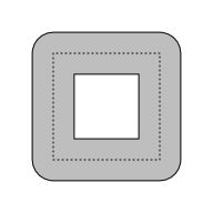
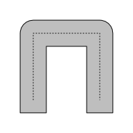
the following code generates a "square donut" by starting with
a rectangle, generating two offset regions (one with positive delta
and one with negative delta), and then subtracting the inner offset region
from the outer offset region.
grid.newpage()
outer <- polyoffsetGrob(r, unit(5, "mm"))
inner <- polyoffsetGrob(r, unit(-5, "mm"))
grid.polyclip(outer, inner, "minus", gp=gpar(fill="grey"))
grid.draw(r)
In all of the examples so far, the offset regions have been created
with rounded corners, but there are other options.
The jointype argument
can be used to select the corner style:
"round" (the default) produces rounded corners.
grid.polyoffset(r, unit(5, "mm"), jointype="round",
                gp=gpar(fill="grey"))
grid.draw(r)

"square" produces bevelled corners.
grid.polyoffset(r, unit(5, "mm"), jointype="square",
                gp=gpar(fill="grey"))
grid.draw(r)

"miter" (or "mitre") produces pointy corners.
grid.polyoffset(r, unit(5, "mm"), jointype="mitre",
                gp=gpar(fill="grey"))
grid.draw(r)
With grid.polylineoffset() we can control the shape
of corners with jointype as above and we can control
the shape of the offset region at the ends of the line or curve
with the endtype argument. .
"openround" (the default)
produces rounded ends at the start and
end of the line.
grid.polylineoffset(l, unit(5, "mm"), endtype="openround",
                    gp=gpar(fill="grey"))
grid.draw(l)

"openbutt" produces square ends at the start
and end of the line.
grid.polylineoffset(l, unit(5, "mm"), endtype="openbutt",
                    gp=gpar(fill="grey"))
grid.draw(l)
"opensquare" produces square ends at an offset from the
start and end of the line.
grid.polylineoffset(l, unit(5, "mm"), endtype="opensquare",
                    gp=gpar(fill="grey"))
grid.draw(l)
There are also two unusual end types that join the end of the line to the start of the line, in which case there are no longer ends to worry about and only the join type matters.
"closedpolygon" converts the line to a polygon
and calculates an offset of the polygon.
grid.polylineoffset(l, unit(5, "mm"), endtype="closedpolygon",
                    gp=gpar(fill="grey"))
grid.draw(l)
"closedline" converts the line to a closed line
and calculates an offset of the line.
grid.polylineoffset(l, unit(5, "mm"), endtype="closedline",
                    gp=gpar(fill="grey"))
grid.draw(l)
This section looks at some more complicated scenarios for calculating offset regions and some lower-level functions that have been added to 'gridGeometry'.
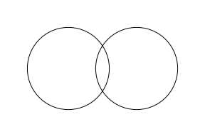
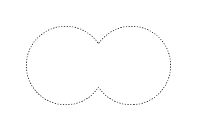
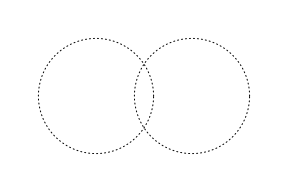
The examples from the previous section have only considered the situation where we are generating an offset region based on a single shape. In this section we consider what happens when we have more than one shape. For example, in the following code we create a 'grid' grob that draws two (overlapping) circles.
circles <- circleGrob(1:2/3, r=.3, gp=gpar(fill=NA))
grid.draw(circles)
The first important point is that 'gridGeometry' will "reduce"
a grob that draws multiple shapes before sending it to
'polyclip'. This happens automatically, but the following
code explicitly performs the reduce, using the
reduceGrob() function, to show what normally happens
by default. In this case, we get a single shape that is the
union of the two circles (drawn as a dotted outline so that
we can add it to the offset region examples below).
circleUnion <- reduceGrob(circles, gp=gpar(lty="dotted", fill=NA))
grid.draw(circleUnion)
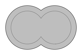
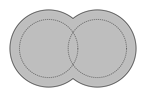
When we calculate an offset region for the two circles we get a single region (shown in grey below). This makes sense because we are actually calculating an offset of the union of the two circles (shown as a dotted outline).
grid.polyoffset(circles, unit(5, "mm"), gp=gpar(fill="grey"))
grid.draw(circleUnion)
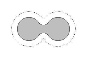
If we use a negative offset, we still get a single region, again because we are offsetting the union of the circles.
grid.polyoffset(circles, unit(-5, "mm"), gp=gpar(fill="grey"))
grid.draw(circleUnion)
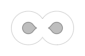
However, if we increase the (negative) offset, it is possible to end up with two regions as the result, even though we are offsetting a single region.
grid.polyoffset(circles, unit(-10, "mm"), gp=gpar(fill="grey"))
grid.draw(circleUnion)
We can also control how the circles are reduced. For example, the following code explicitly reduces the circles using a "flatten" operator, which keeps the circles as two separate circles.
circleFlatten <- reduceGrob(circles, op="flatten",
                            gp=gpar(lty="dotted", fill=NA))
grid.draw(circleFlatten)
When we specify an explicit reduce="flatten" to
grid.polyoffset(), we can end up sending
multiple shapes to 'polyclip'.
The following code generates an offset region based on two separate circles. The result is a single region, just the same as when we offset the union of the circles, because the offset regions of the two circles overlap.
grid.polyoffset(circles, unit(5, "mm"), reduce="flatten", gp=gpar(fill="grey"))
grid.draw(circleFlatten)
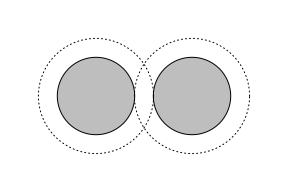
However, if we use a negative offset, the result is two separate regions (because the offset regions of the two circles do not overlap).
grid.polyoffset(circles, unit(-5, "mm"), reduce="flatten", gp=gpar(fill="grey"))
grid.draw(circleFlatten)
In summary, it is possible to start with either a single shape or multiple shapes and end up with either a single shape or multiple shapes, depending on how (or whether) we reduce the input shapes and on whether the resulting offset regions (if there are more than one) overlap each other.
In the previous sections, we have demonstrated functions that allow us to provide 'grid' grobs as input and obtain grobs as output. The 'gridGeometry' package also provides a lower-level interface that just works with coordinates rather than grobs.
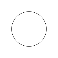
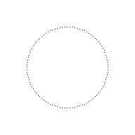
As an example of working at a lower level, consider the simple circle shape shown below.
c <- circleGrob(r=.3)
grid.draw(c)
Suppose we want to create a "donut" shape based on this circle.
We need an offset larger than the circle and an offset smaller
than the circle, but because the circle is a closed shape,
we can only use
grid.polyoffset() to produce either a larger circle
or a smaller circle.
The following code uses the lower-level xyListFromGrob()
function to generate an xy-list (a list of sets of x/y coordinates)
from the circle grob.
pts <- xyListFromGrob(c)
pts
  [[1]]
  x: 1.6 1.598816 1.595269 ... [100 values]
  y: 1 1.037674 1.0752 ... [100 values]
The result is a set of points around a circle.
grid.points(pts[[1]]$x, pts[[1]]$y, default.units="in", pch=".")
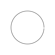
Now that we are dealing with a lower-level set of coordinates, rather than
higher-level grob, we can treat these coordinates as an open shape
rather than a closed shape. For example, the following code
uses the xyListToLine() function to generate a series of line
segments that go most of the way, but not all of the way, around the circle
(there is a small gap on the right of the circle).
grid.draw(xyListToLine(pts))
The next code also treats the coordinates as an open shape,
but it calls the polylineoffset() function
to generate a set of offset coordinates. This creates an offset
on both sides of the line and, because we specify
endtype="closedline", does so all of the way around
the circle.
The result is still just coordinates, but it is now a list of 2 sets
of x/y coordinates (the outer edge of the donut and the inner edge
of the donut).
offsetpts <- polylineoffset(pts, delta=unit(2, "mm"), endtype="closedline")
offsetpts
  [[1]]
  [[1]]$x
    [1] 1.0401476 1.0450844 1.0826100 1.0875176 1.1247465 1.1296054 1.1663906 1.1711817 1.2073780
   [10] 1.2120825 1.2475470 1.2521462 1.2867391 1.2912149 1.3247995 1.3291342 1.3615781 1.3657546
   [19] 1.3969297 1.4009316 1.4307148 1.4345262 1.4628001 1.4664060 1.4930589 1.4964450 1.5213718
   [28] 1.5245249 1.5476271 1.5505347 1.5717212 1.5743717 1.5935590 1.5959420 1.6130542 1.6151604
   [37] 1.6301300 1.6319510 1.6447190 1.6462476 1.6567636 1.6579937 1.6662162 1.6671431 1.6730396
   [46] 1.6736595 1.6772067 1.6775173 1.6787013 1.6787013 1.6775173 1.6772067 1.6736595 1.6730396
   [55] 1.6671431 1.6662162 1.6579937 1.6567636 1.6462476 1.6447190 1.6319510 1.6301300 1.6151604
   [64] 1.6130542 1.5959420 1.5935590 1.5743717 1.5717212 1.5505347 1.5476271 1.5245249 1.5213718
   [73] 1.4964450 1.4930589 1.4664060 1.4628001 1.4345262 1.4307148 1.4009316 1.3969297 1.3657546
   [82] 1.3615781 1.3291342 1.3247995 1.2912149 1.2867391 1.2521462 1.2475470 1.2120825 1.2073780
   [91] 1.1711817 1.1663906 1.1296054 1.1247465 1.0875176 1.0826100 1.0450844 1.0401476 1.0024733
  [100] 0.9975267 0.9598524 0.9549156 0.9173900 0.9124824 0.8752535 0.8703946 0.8336094 0.8288183
  [109] 0.7926220 0.7879175 0.7524530 0.7478538 0.7132609 0.7087851 0.6752005 0.6708658 0.6384219
  [118] 0.6342454 0.6030703 0.5990684 0.5692852 0.5654738 0.5371999 0.5335940 0.5069411 0.5035550
  [127] 0.4786282 0.4754751 0.4523729 0.4494653 0.4282788 0.4256283 0.4064410 0.4040580 0.3869458
  [136] 0.3848396 0.3698700 0.3680490 0.3552810 0.3537524 0.3432364 0.3420063 0.3337838 0.3328569
  [145] 0.3269604 0.3263405 0.3227933 0.3224827 0.3212987 0.3212987 0.3224827 0.3227933 0.3263405
  [154] 0.3269604 0.3328569 0.3337838 0.3420063 0.3432364 0.3537524 0.3552810 0.3680490 0.3698700
  [163] 0.3848396 0.3869458 0.4040580 0.4064410 0.4256283 0.4282788 0.4494653 0.4523729 0.4754751
  [172] 0.4786282 0.5035550 0.5069411 0.5335940 0.5371999 0.5654738 0.5692852 0.5990684 0.6030703
  [181] 0.6342454 0.6384219 0.6708658 0.6752005 0.7087851 0.7132609 0.7478538 0.7524530 0.7879175
  [190] 0.7926220 0.8288183 0.8336094 0.8703946 0.8752535 0.9124824 0.9173900 0.9549156 0.9598524
  [199] 0.9975267 1.0024733

  [[1]]$y
    [1] 0.3224827 0.3227933 0.3263405 0.3269604 0.3328569 0.3337838 0.3420063 0.3432364 0.3537524
   [10] 0.3552810 0.3680490 0.3698700 0.3848396 0.3869458 0.4040580 0.4064410 0.4256283 0.4282788
   [19] 0.4494653 0.4523729 0.4754751 0.4786282 0.5035550 0.5069411 0.5335940 0.5371999 0.5654738
   [28] 0.5692852 0.5990684 0.6030703 0.6342454 0.6384219 0.6708658 0.6752005 0.7087851 0.7132609
   [37] 0.7478538 0.7524530 0.7879175 0.7926220 0.8288183 0.8336094 0.8703946 0.8752535 0.9124824
   [46] 0.9173900 0.9549156 0.9598524 0.9975267 1.0024733 1.0401476 1.0450844 1.0826100 1.0875176
   [55] 1.1247465 1.1296054 1.1663906 1.1711817 1.2073780 1.2120825 1.2475470 1.2521462 1.2867391
   [64] 1.2912149 1.3247995 1.3291342 1.3615781 1.3657546 1.3969297 1.4009316 1.4307148 1.4345262
   [73] 1.4628001 1.4664060 1.4930589 1.4964450 1.5213718 1.5245249 1.5476271 1.5505347 1.5717212
   [82] 1.5743717 1.5935590 1.5959420 1.6130542 1.6151604 1.6301300 1.6319510 1.6447190 1.6462476
   [91] 1.6567636 1.6579937 1.6662162 1.6671431 1.6730396 1.6736595 1.6772067 1.6775173 1.6787013
  [100] 1.6787013 1.6775173 1.6772067 1.6736595 1.6730396 1.6671431 1.6662162 1.6579937 1.6567636
  [109] 1.6462476 1.6447190 1.6319510 1.6301300 1.6151604 1.6130542 1.5959420 1.5935590 1.5743717
  [118] 1.5717212 1.5505347 1.5476271 1.5245249 1.5213718 1.4964450 1.4930589 1.4664060 1.4628001
  [127] 1.4345262 1.4307148 1.4009316 1.3969297 1.3657546 1.3615781 1.3291342 1.3247995 1.2912149
  [136] 1.2867391 1.2521462 1.2475470 1.2120825 1.2073780 1.1711817 1.1663906 1.1296054 1.1247465
  [145] 1.0875176 1.0826100 1.0450844 1.0401476 1.0024733 0.9975267 0.9598524 0.9549156 0.9173900
  [154] 0.9124824 0.8752535 0.8703946 0.8336094 0.8288183 0.7926220 0.7879175 0.7524530 0.7478538
  [163] 0.7132609 0.7087851 0.6752005 0.6708658 0.6384219 0.6342454 0.6030703 0.5990684 0.5692852
  [172] 0.5654738 0.5371999 0.5335940 0.5069411 0.5035550 0.4786282 0.4754751 0.4523729 0.4494653
  [181] 0.4282788 0.4256283 0.4064410 0.4040580 0.3869458 0.3848396 0.3698700 0.3680490 0.3552810
  [190] 0.3537524 0.3432364 0.3420063 0.3337838 0.3328569 0.3269604 0.3263405 0.3227933 0.3224827
  [199] 0.3212987 0.3212987


  [[2]]
  [[2]]$x
    [1] 0.9672723 0.9346737 0.9023329 0.8703776 0.8389339 0.8081258 0.7780749 0.7488999 0.7207158
   [10] 0.6936340 0.6677612 0.6431997 0.6200463 0.5983923 0.5783234 0.5599186 0.5432506 0.5283852
   [19] 0.5153810 0.5042894 0.4951541 0.4880113 0.4828890 0.4798075 0.4787790 0.4798075 0.4828890
   [28] 0.4880113 0.4951541 0.5042894 0.5153810 0.5283852 0.5432506 0.5599186 0.5783234 0.5983923
   [37] 0.6200463 0.6431997 0.6677612 0.6936340 0.7207158 0.7488999 0.7780749 0.8081258 0.8389339
   [46] 0.8703776 0.9023329 0.9346737 0.9672723 1.0000000 1.0327277 1.0653263 1.0976671 1.1296224
   [55] 1.1610661 1.1918742 1.2219251 1.2511001 1.2792842 1.3063660 1.3322388 1.3568003 1.3799537
   [64] 1.4016077 1.4216766 1.4400814 1.4567494 1.4716148 1.4846190 1.4957106 1.5048459 1.5119887
   [73] 1.5171110 1.5201925 1.5212210 1.5201925 1.5171110 1.5119887 1.5048459 1.4957106 1.4846190
   [82] 1.4716148 1.4567494 1.4400814 1.4216766 1.4016077 1.3799537 1.3568003 1.3322388 1.3063660
   [91] 1.2792842 1.2511001 1.2219251 1.1918742 1.1610661 1.1296224 1.0976671 1.0653263 1.0327277
  [100] 1.0000000

  [[2]]$y
    [1] 0.4798075 0.4828890 0.4880113 0.4951541 0.5042894 0.5153810 0.5283852 0.5432506 0.5599186
   [10] 0.5783234 0.5983923 0.6200463 0.6431997 0.6677612 0.6936340 0.7207158 0.7488999 0.7780749
   [19] 0.8081258 0.8389339 0.8703776 0.9023329 0.9346737 0.9672723 1.0000000 1.0327277 1.0653263
   [28] 1.0976671 1.1296224 1.1610661 1.1918742 1.2219251 1.2511001 1.2792842 1.3063660 1.3322388
   [37] 1.3568003 1.3799537 1.4016077 1.4216766 1.4400814 1.4567494 1.4716148 1.4846190 1.4957106
   [46] 1.5048459 1.5119887 1.5171110 1.5201925 1.5212210 1.5201925 1.5171110 1.5119887 1.5048459
   [55] 1.4957106 1.4846190 1.4716148 1.4567494 1.4400814 1.4216766 1.4016077 1.3799537 1.3568003
   [64] 1.3322388 1.3063660 1.2792842 1.2511001 1.2219251 1.1918742 1.1610661 1.1296224 1.0976671
   [73] 1.0653263 1.0327277 1.0000000 0.9672723 0.9346737 0.9023329 0.8703776 0.8389339 0.8081258
   [82] 0.7780749 0.7488999 0.7207158 0.6936340 0.6677612 0.6431997 0.6200463 0.5983923 0.5783234
   [91] 0.5599186 0.5432506 0.5283852 0.5153810 0.5042894 0.4951541 0.4880113 0.4828890 0.4798075
  [100] 0.4787790
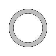
As a final step,
we can use xyListToPath() to convert the coordinates
back to a grob for drawing.
donut <- xyListToPath(offsetpts, gp=gpar(fill="grey"))
grid.draw(donut)
As with the original grid.polyclip() function,
the new functions in 'gridGeometry' have value as an additional
tool for creating shapes in R graphics. This is potentially useful
because new (graphical) tools help us to
think about (graphical) problems in new ways and allow us to
come up with new (graphical) solutions.
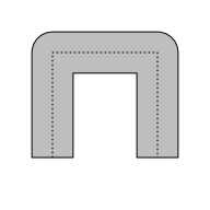
As a simple example, consider the more complicated "gear" shape shown below. We saw in the introduction how easy it is to create the "teeth" around the outside of the gear shape, but how can we create the wedge-shaped holes in the interior of the gear shape, particularly with rounded corners on each wedge?
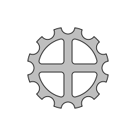
With the concept of offset regions (with rounded corners) in our
toolbox, it is easier to think of ways to generate this shape.
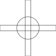
To start with, we will use grid.polyclip() to
subtract horizontal and vertical bars from a medium-sized circle.
The following code shows the circles and bars that we are working with.
medC <- circleGrob(r=.2, gp=gpar(fill=NA))
hbar <- rectGrob(height=.1, gp=gpar(fill=NA))
vbar <- rectGrob(width=.1, gp=gpar(fill=NA))
grid.draw(medC)
grid.draw(hbar)
grid.draw(vbar)
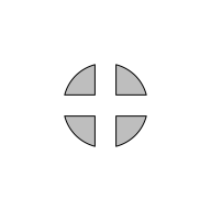
The following code subtracts the bars from the medium-sized circle, which leaves four wedges.
wedges <- polyclipGrob(medC, gList(hbar, vbar), "minus",
                         gp=gpar(fill="grey"))
grid.draw(wedges)
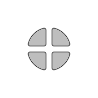
The next code generates offset regions based on the four wedges. This produces the curved corners on the wedges.
roundedWedges <- polyoffsetGrob(wedges, unit(1, "mm"),
                                gp=gpar(fill="grey"))
grid.draw(roundedWedges)
The final step is to subtract those wedges from the large circle that we started with in the introduction (as well as subtracting the small circles to make the teeth).
grid.polyclip(bigC, gList(littleC, roundedWedges), "minus",
              gp=gpar(fill="grey"))
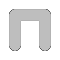
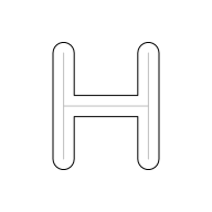
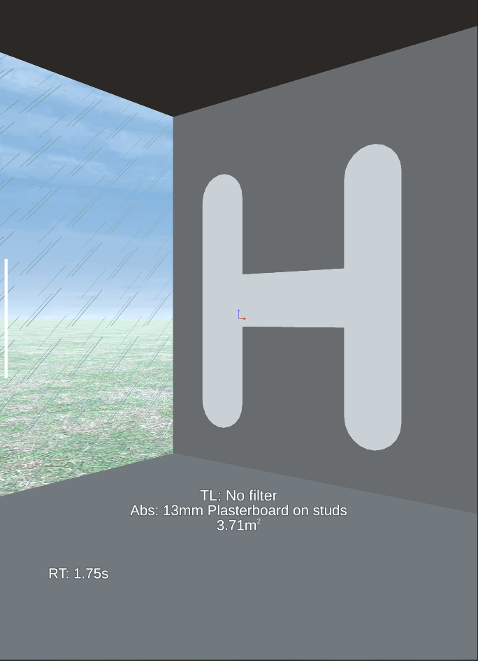
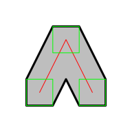
The first author has also made use of the new offset facilities in 'gridGeometry' to create shapes for an acoustic similation app called AiHear (Beresford and Wong, 2022). For example, the offset facilities made it easy to create an "H" shape, with rounded ends on the verticals, as shown below.
The relatively complex final outline is not described directly. Instead, a simple series of straight lines is described (shown in grey below) and then the final result is obtained from the union of the offset regions based on the straight lines.
l1 <- linesGrob(x=rep(0.3, 2), y=c(0.25, 0.75), gp=gpar(col="grey"))
l2 <- linesGrob(x=rep(0.7, 2), y=c(0.25, 0.75), gp=gpar(col="grey"))
l3 <- linesGrob(x=c(0.3, 0.7), y=rep(0.5, 2), gp=gpar(col="grey"))
l <- gList(l1, l2, l3)
grid.draw(l)
grid.polylineoffset(l, 0.05, endtype = "openround", jointype = "round",
                    gp=gpar(fill=NA))
This is a nice example of a simple solution to a problem only becoming apparent once the idea of offset regions has been introduced. The image below shows the "H" that was created in R being used in the AiHear app.
An example of a
statistical graphics application
is the creation of non-standard data symbols.
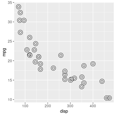
For example, the code below draws "donut" data symbols
in a 'ggplot2' plot (Wickham, 2016; the 'gggrid' package is
used to combine low-level 'grid' drawing with the 'ggplot2' plot;
Murrell, 2022b).
This code builds a "donutGrob" object for each data point
and defines a makeContent() method for "donutGrob"s
so that the calculation of offset regions happens when the
data points are drawn (rather than when they are created).
donutGrob <- function(x, y) {
    gTree(x=x, y=y, cl="donutGrob")
}
makeContent.donutGrob <- function(x) {
    circles <- mapply(circleGrob, x$x, x$y, MoreArgs=list(r = unit(1.5, "mm")),
                      SIMPLIFY=FALSE)
    pts <- lapply(circles, xyListFromGrob)
    offsetpts <- lapply(pts, polylineoffset, delta=unit(.5, "mm"),
                        endtype="closedline")
    donuts <- lapply(offsetpts, xyListToPath, gp=gpar(fill="white"))
    setChildren(x, do.call(gList, donuts))
}
donut <- function(data, coords) {
    donutGrob(coords$x, coords$y)
}
library(gggrid)
ggplot(mtcars) +
    grid_panel(donut, aes(x=disp, y=mpg, colour=as.factor(am), fill=hp))
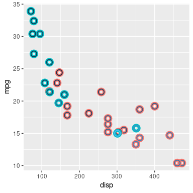
The difference between drawing donut symbols and just open circles using a thick line width is that the donuts have a separate (interior and exterior) border and fill. This is emphasised in the following variation where the donut borders are coloured to represent whether cars are manual (blueish) or automatic (reddish) and the donut fills represent the horsepower (dark to light). The manual car with the highest horsepower is clearly visible.
donutGrob <- function(x, y, colour, fill) {
    gTree(x=x, y=y, colour=colour, fill=fill, cl="donutGrob")
}
cook <- function(offsetpts, colour, fill) {
    xyListToPath(offsetpts, gp=gpar(col=colour, fill=fill, lwd=2))
}
makeContent.donutGrob <- function(x) {
    circles <- mapply(circleGrob, x$x, x$y, MoreArgs=list(r = unit(1.5, "mm")),
                      SIMPLIFY=FALSE)
    pts <- lapply(circles, xyListFromGrob)
    offsetpts <- lapply(pts, polylineoffset, delta=unit(.5, "mm"),
                        endtype="closedline")
    donuts <- mapply(cook, offsetpts, x$colour, x$fill, SIMPLIFY=FALSE)
    setChildren(x, do.call(gList, donuts))
}
donut <- function(data, coords) {
    donutGrob(coords$x, coords$y, coords$colour, coords$fill)
}
ggplot(mtcars) +
    grid_panel(donut, aes(x=disp, y=mpg, colour=as.factor(am), fill=hp))
In addition to the functions for generating offset regions,
support has also been added to the 'gridGeometry' package for generating
Minkowski Sums.
The main function is grid.minkowski(), which takes
two shapes, a "pattern" and a "path", and generates a new shape
by "adding" the pattern to the path.
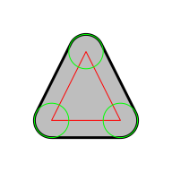
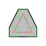
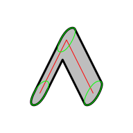
For certain cases, a Minkowski Sum generates a result just like an offset region. For example, the following code adds a circle pattern to a triangular path. This is done by adding the circle to every location on the triangle. The result (black outline with grey fill) is like an offset region for the triangle (the original triangle is shown in red and examples of the circle being added to the vertices of the triangle are shown in green).
circle <- circleGrob(0, 0, r=.1, gp=gpar(col="green", fill=NA))
triangle <- polygonGrob(c(.3, .5, .7), c(.3, .7, .3),
                        gp=gpar(col="red", fill=NA))
grid.minkowski(circle, triangle, gp=gpar(lwd=3, fill="grey"))
However, the pattern can be any shape, so the final result is more general than the offset regions described previously. For example, the following code adds a rectangle pattern to the triangle.
rect <- rectGrob(0, 0, width=.2, height=.2, gp=gpar(col="green", fill=NA))
grid.minkowski(rect, triangle, gp=gpar(lwd=3, fill="grey"))
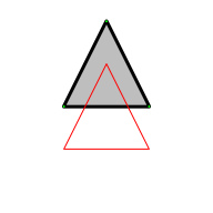
The examples so far have used a pattern that is centred on (0, 0), so the result is just an expanded version of the original path. However, the pattern can also induce a translation of the path. As an extreme example, the following code adds a tiny circle to the triangle. The circle has almost zero width so it does not expand the triangle, but the circle is at (0, .2) so the result is translated vertically.
pt <- circleGrob(0, .2, r=0.001, gp=gpar(col="green"))
grid.minkowski(pt, triangle, gp=gpar(lwd=3, fill="grey"))
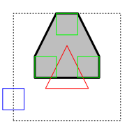
In full generality, the Minkowski Sum produces the sum of all vectors within the pattern and the path. This is shown in the following diagram: the region that we are drawing within is represented by a dotted rectangle, with the origin, (0, 0), at the bottom-left corner of the dotted rectangle; the pattern, a rectangle, is drawn in blue to show that it is offset vertically from the origin; the path, a triangle, is drawn in red; and examples of the pattern being added to the path (at the triangle vertices) are drawn in green. The final Minkowski Sum is the black region with a grey fill.
smallRect <- rectGrob(0, .2, width=.2, height=.2, gp=gpar(col="green", fill=NA))
grid.minkowski(smallRect, triangle, gp=gpar(lwd=3, fill="grey"))
The path can also be an open shape. For example, the following code adds a rectangle pattern to a line.
line <- linesGrob(c(.3, .5, .7), c(.3, .7, .3),
                  gp=gpar(col="red"))
grid.minkowski(rect, line, gp=gpar(lwd=3, fill="grey"))
This usage allows us to create shapes by stroking a path with a pen, in the spirit of METAFONT (Knuth, 1989) or METAPOST (Hobby, 1998). For example, the following code creates an ellipsoid pen (pattern) and strokes the line with that pen (adds the pattern to the path).
pen <- xsplineGrob(c(-.1, 0, .1, 0), c(-.1, .1, .1, -.1),
                   open=FALSE, shape=1,
                   gp=gpar(col="green", fill=NA))
grid.minkowski(pen, line, gp=gpar(lwd=3, fill="grey"))
New functions in the 'gridGeometry' package provide access
to more of the facilities in the 'polyclip' package. The main interface
for generating offset regions
is provided by grid.polyoffset() for closed
shapes and grid.polylineoffset() for open shapes.
There is also a new interface for generating Minkowski Sums
via the grid.minkowski() function.
The examples and discussion in this report relate to version 0.4-0 of the 'gridGeometry' package.
This report was generated within a Docker container (see Resources section below).
Wong, J., and Murrell, P. (2022). "Offsetting Lines and Polygons in 'grid'" Technical Report 2022-03, Department of Statistics, The University of Auckland. Version 1. [ bib | DOI | http ]
This document
by Paul
Murrell is licensed under a Creative
Commons Attribution 4.0 International License.