 http://orcid.org/0000-0002-3224-8858
by Paul Murrell
http://orcid.org/0000-0002-3224-8858
Version 3: Monday 22 May 2023
Version 1: Original publication (Monday 15 November 2021).
Version 2: Removed "Accumulating transformations"; added "The vp argument"; added "Appendix" (Monday 30 May 2022).
Version 3: Update behaviour of Porter-Duff compositing operators; quartz() support added; removed "Appendix".

This document
by Paul
Murrell is licensed under a Creative
Commons Attribution 4.0 International License.
This document describes an expansion of the R graphics engine to support a number of new graphical features: isolated groups, compositing operators, and affine transformations.
These features are available from R version 4.2.0.
R users wanting to try out the new graphics features should start with the User API Section, which provides a quick introduction to the new R-level interface.
Maintainers of R packages that provide R graphics devices should read the Device API Section, which provides a description of the required changes to R graphics devices.
These new graphics features have not (yet) been implemented for
all of the graphics devices provided by the 'grDevices'
package. Devices that do support the new features are the
pdf() graphics device,
the quartz() graphics device (from R 4.3.0),
and Cairo graphics devices:
x11(type="cairo"), cairo_pdf(),
cairo_ps(), png(type="cairo"),
jpeg(type="cairo"), tiff(type="cairo"),
and svg().
The remainder of the graphics
devices in 'grDevices' will run, but will (silently) not produce
the correct output. Graphics devices from other R packages should
be reinstalled and will not produce the correct output until
(or unless)
the package maintainer adds support.
Changes to the graphics engine in R 4.1.0 added support for
gradient and pattern fills, clipping paths, and masks
(Murrell, 2020b).
One way to think of those changes is that they
created an R interface to some of the more advanced graphical features
of specific R graphics devices - graphics devices that are based on
sophisticated graphics systems, like the pdf() device
that is based on the Adobe Portable Document Format
(Adobe Systems Incorporated, 2001) and the graphics
devices based on the Cairo graphics library (Packard et al., 2021).
This document describes another step along that path, by adding
an R interface to work with "groups" of graphical objects.
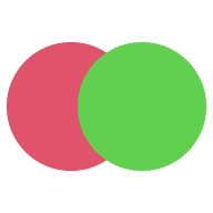
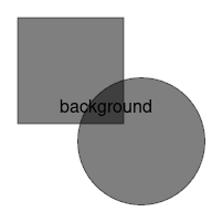
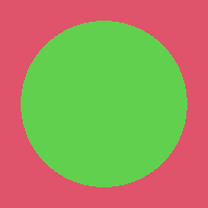
As a simple example of the increased sophistication provided by the new features, consider the following code, which draws two opaque filled circles that partially overlap each other on top of a piece of text (the text is completely obscured).
library(grid)
grid.text("background")
c <- circleGrob(1:2/3, r=.3, gp=gpar(col=2:3, fill=2:3))
grid.draw(c)
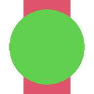
We will now draw the same circles (and text), but this time in a viewport with a semitransparency mask.
grid.text("background")
mask <- rectGrob(gp=gpar(col=NA, fill=rgb(0,0,0,.5)))
pushViewport(viewport(mask=mask))
grid.draw(c)
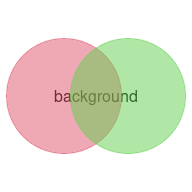
The result is that each circle is drawn with the mask applied, so each circle becomes semitransparent. The circles overlap so we get a region where the first circle is partially visible beneath the second circle. The text is also visible beneath the circles.
Now consider the following code, which draws the circles, but this time as a "group", again in a viewport with a semitransparency mask.
grid.text("background")
pushViewport(viewport(mask=mask))
grid.group(c)
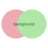
The difference is that the opaque circles are drawn together first as an isolated group, with the green circle partially obscuring the red circle (as in the original drawing), and only then is the mask applied. The mask has been applied to the result of drawing the group of circles rather than being applied to each circle as it is drawn. The text is again visible beneath the circles to show that the area of intersection between the circles is only the green circle made semitransparent.
This captures the essence of the new graphics features that are provided in this report: we get to draw a group of objects in isolation before adding the group to the overall image.
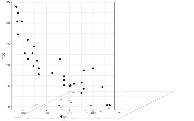
The image below provides a more dramatic demonstration. Here we have a 'ggplot2' plot (Wickham, 2016) treated as an isolated group. The group has been drawn twice: once as it would appear normally (upright) and once with a shear transformation applied (to give the impression of a shadow that is cast by the plot). This hints at the fact that, once we have defined a group of shapes in isolation, there are a number of new effects that we can achieve. The code for the image below will be shown later once we have a better idea of how the new graphics functions work.

The User API Section provides simple examples that demonstrate all of the new user-level features and demonstrate some of the effects that can be obtained from them.
The Section Exploring the new features goes into more detail about how the new user-level functions work. This is not necessary for simple usage, but there are useful details for more sophisticated use of the new features.
The new features are only implemented on a few of the standard
R graphics devices so far (the pdf() device and
the devices based on the Cairo graphics system); the
Device API Section describes the interface that
graphics devices must implement if they want to support these
features.
The simple overlapping-circles examples above are representative of most examples in this report; they are simple demonstrations of graphical features, with no obvious connection to data visualisation. The main motivation for adding the new features to the R graphics engine is to reduce the need for users to have to manually tweak R graphics output in other systems like Adobe Illustrator. In other words, the aim of these changes is to encourage users to generate graphical output entirely in code, with all of the benefits of reproducibility, sharing, version control etc that come with working entirely in code. Direct applications of these features to data visualisation will hopefully follow as users and developers experiment with the new possibilities.
The first new function to describe is the grid.group()
function. As shown in the Introduction, this function
takes a 'grid' grob, renders it in isolation, and then
combines it with the main image.
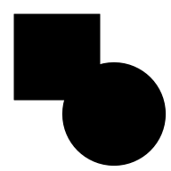
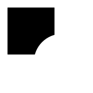
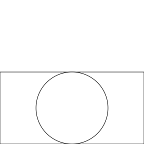
The isolated drawing can be arbitrarily complex, involving multiple grobs and viewports, by providing a gTree as the first argument. For example, the following code draws a rectangle and a circle as a group.
r <- rectGrob(1/3, 2/3, width=.5, height=.5, gp=gpar(fill="black"))
c <- circleGrob(2/3, 1/3, r=.3, gp=gpar(fill="black"))
gt <- gTree(children=gList(r, c))
grid.group(gt)
The following code draws the entire gTree from a 'ggplot2' plot as a group.
library(ggplot2)
gg <- ggplotGrob(ggplot(mtcars) + geom_point(aes(disp, mpg)))
grid.group(gg)

The above results are exactly the same as the results we would get by just drawing the grobs normally, as the code below shows for the simple rectangle-plus-circle example.
grid.draw(gt)

We get the same result in the examples above because, when we draw the shapes as a group, we begin with a temporary transparent canvas, we draw the group on this temporary canvas, and then the result is drawn on top of any previous drawing in the main image However, there are several ways in which we can vary that situation.
If we enforce a mask (in the main image), the results of drawing normally and drawing as a group are no longer the same. This was the first example shown in the introduction. The code below repeats the example with the rectangle and circle, but now with a mask in place. Some text is drawn in the background so that we can more easily see the transparency of the shapes.
First we draw normally. The text is drawn in the background, then we push a viewport that enforces a semitransparent mask. The rectangle is drawn and, because of the mask, it is semitransparent, so we can see the text beneath it. Then the circle is drawn and it is also semitransparent, so we can see the text beneath it and, where the circle and the rectangle overlap, we can also see the rectangle beneath the cirlce.
grid.text("background")
pushViewport(viewport(mask=mask))
grid.draw(gt)
Now we draw the shapes as a group. As before, the text is drawn and a viewport is pushed to enforce a mask. However, the rectangle and circle are now drawn as an isolated group, as a separate step. The result of drawing the rectangle and circle is then added to the main image, with the mask now in effect, so we get the result of drawing the rectangle and circle with no mask (the opaque union of the rectangle and circle) added to the main image using a mask, which produces a semitransparent union of the rectangle and circle. We can see the text beneath, but there is no visible overlap between the rectangle and circle.
grid.text("background")
pushViewport(viewport(mask=mask))
grid.group(gt)

Another way that we can get a different result from drawing shapes in a group is that we can vary how shapes are drawn on top of each other (in the group).
By default, each new shape is drawn on top of any previous drawing,
with the new shape obscuring previous drawing where there is any
overlap. The grid.group()
function has two further arguments, op and dst
(the first argument is called src),
which allow us to combine new shapes with previous shapes in
a variety of ways.
The dst argument is a 'grid' grob (like the
src argument) and this is drawn first.
The op argument selects a "compositing operator"
and this specifies how the src grob is combined with
the dst. The default op value is
"over".
The following code uses the same
simple shapes in the group as before (a rectangle and a circle),
but now, within the group, we draw the rectangle first
(as dst)
and then the circle (as src),
using a "dest.out" operator.
With this operator, the new shape removes the previous drawing
wherever there is an overlap. In this case,
drawing the circle over the rectangle takes a bite out of
the bottom-right corner of
the rectangle. With the "dest.out" operator,
the src is not drawn at all.
grid.group(c, "dest.out", r)
By default, the dst is a fully transparent rectangle,
but we can easily specify a different "backdrop" for a group.
The following code specifies a grey filled rectangle as the
dst and then draws the gTree consisting of the
rectangle and the circle on top, using a "dest.out"
operator. The result is a hole punched in the grey rectangle
based on the black rectangle and the black circle.
To show that the result of drawing this group is NOT the
same as drawing a white rectangle and a white circle on top
of the grey rectangle, we first drew some text in the main image;
when the group is drawn on top of the main image we can see
the text through the hole that the rectangle and circle
have punched in the grey rectangle.
grid.text("reveal", gp=gpar(cex=4))
grid.group(gt, "dest.out", rectGrob(gp=gpar(col= NA, fill="grey")))

All of the compositing
operators supported by the Cairo
graphics system are provided
(including the standard Porter-Duff operators;
Porter and Duff, 1984),
but only a subset of these are
supported on the PDF graphics device. In the PDF language,
the compositing operators are called "blend modes"; the default
"over" operator corresponds to "Normal" blend mode
and several other operators correspond to
the other PDF blend modes,
but the "dest.out" operator, for example, has no
corresponding blend mode. Where there is no correspondence,
the PDF device falls back to "Normal" blend mode.
The full list of available operators are shown below.
   [1] "clear"       "source"      "over"        "in"          "out"         "atop"
   [7] "dest"        "dest.over"   "dest.in"     "dest.out"    "dest.atop"   "xor"
  [13] "add"         "saturate"    "multiply"    "screen"      "overlay"     "darken"
  [19] "lighten"     "color.dodge" "color.burn"  "hard.light"  "soft.light"  "difference"
  [25] "exclusion"
In addition to grid.group(), there are two other
new functions: grid.define() and grid.use().
The purpose of these functions is to separate the definition of
a group from its use. This allows us to reuse a group multiple times
from a single definition.
As an example, the following code defines a group consisting of a circle and a rectangular, similar to the one we have been using, but smaller.
r2 <- rectGrob(width=unit(1, "cm"), height=unit(1, "cm"),
               hjust=.75, vjust=.25,
               just=c("right", "bottom"),
               gp=gpar(fill="black"))
c2 <- circleGrob(x=unit(.5, "npc") + unit(.5, "cm"),
                 y=unit(.5, "npc") - unit(.5, "cm"),
                 r=unit(.67, "cm"),
                 gp=gpar(fill="black"))
gt2 <- gTree(children=gList(r2, c2))
grid.group(gt2)

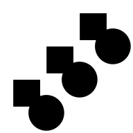
In the following code, we first call grid.define()
to define the group and give it a name, "group1".
This does not draw the group, it just defines the group
on the graphics device.
We then call grid.use() with the name of the group
we want to use, and this draws the group.
This produces the drawing in the centre of the page, just like
grid.group() did and
demonstrates that grid.group() is really
just a wrapper for grid.define() and
grid.use().
The interesting part happens next. We push a viewport in a
different location on the page (the bottom-left corner)
and call grid.use()
again. This draws the group in a different location on the page.
Then we repeat the dose to draw the group in yet another location
(the top-right corner).
grid.define(gt2, name="group1")
grid.use("group1")
pushViewport(viewport(.25, .25, gp=gpar(col=2)))
grid.use("group1")
popViewport()
pushViewport(viewport(.75, .75, gp=gpar(col=3)))
grid.use("group1")
popViewport()
One potential benefit of this feature is efficiency on the graphics device. For example, the PDF device records the group definition only once and then can just refer to the definition every time the group is drawn.
A more interesting detail about the example above is that the
grid.use calls are applying a translation to
the group to redraw it in different locations on the page.
This opens up a whole new world of possibilities.
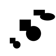
The following code performs the same two initial steps as the last example: we define a group and the use it. This draws the group in the centre of the page. However, the next step is different. Here we push a viewport that is in the bottom-left corner of the page and is smaller than the original viewport that we defined the group in. This difference in both viewport location and size induces both a translation due to the different location of the viewport and a scaling transformation due to the different size of the viewport. The result is that the original group is drawn scaled down (and translated). The final step demonstrates the scaling more dramatically. This time we have a viewport at a different location (top-right) and with a different size and with a different aspect ratio (twice as wide as it is high). The result is that the original group is drawn scaled and distorted (the circle has become an ellipse).
grid.define(gt2, name="group1")
grid.use("group1")
pushViewport(viewport(.25, .25, width=.5, height=.5))
grid.use("group1")
popViewport()
pushViewport(viewport(.75, .75, height=.5))
grid.use("group1")
popViewport()
It is important to note that these transformations are different
from what would normally happen when we draw 'grid' objects.
The transformations are happening on the device rather than in 'grid'.
The following code is identical to the code above except that
it calls grid.draw(), which draws the grob gt2
normally, rather than grid.use(), which draws the group
"group1" that was defined based on the grob gt2.
When we draw
gt2 normally, it remains the same size, regardless
of which viewport we draw it in, because
the width and height of the rectangle and the radius of the
circle were specified in absolute units (cm).
grid.define(gt2, name="group1")
grid.draw(gt2)
pushViewport(viewport(.25, .25, width=.5, height=.5))
grid.draw(gt2)
popViewport()
pushViewport(viewport(.75, .75, height=.5))
grid.draw(gt2)
popViewport()

The behaviour of affine transformations is explored in more detail in the next section, along with several other aspects of drawing groups.
This section goes into further detail about how the new graphics engine features work. It is not necessary for basic usage, but is required to achieve more complex results and may be helpful to understand the output when an unexpected result occurs.
When we define a group with grid.define(),
we give it a name, which we can then use
to refer to the group in a call to grid.use().
These names are unique per device.
If we define a new group with the same name as an existing
group, the new group replaces the old group. For example,
the following code defines a group called "a"
based on a rectangle, then defines another group called
"a" based on a circle. When we subsequently
use the group
called "a", the result is a circle.
grid.define(rectGrob(), name="a")
grid.define(circleGrob(), name="a")
grid.use("a")
Group definitions are usually erased at the start of a new page.
However, the grid.newpage() function has a
clearGroups argument. If that is set to FALSE
then a group can be defined on one page and reused on another page.
The grobs within a group may specify some explicit graphical parameter settings and the group will inherit graphical parameter settings from the context in which the group is defined. However, both explicit and inherited settings are then fixed for any use of the group.
For example, in the code below, we first push a viewport (on the left) that has an explicit line width (2) and colour (red). We draw a rectangle with no explicit graphical parameter settings to show that, in normal 'grid' drawing, the settings from the viewport provide defaults for any drawing within the viewport; the rectangle is drawn with a thin red border. Within the same viewport, we also define a group based on a circle with an explicit line width setting (5). This group ignores the line width default, because it has its own explicit line width, but inherits the default colour red. When we then use the group, we get a (thick) red circle. Next, we push a new viewport (on the right) with green as the default colour and a thicker default line width (5). As before, when we draw a rectangle with no explicit graphical parameter settings, it uses the defaults from the viewport, and we get a thick green rectangle. However, when we reuse the group within this viewport, the circle retains the (explicit) line width and the (inherited) colour from when it was defined and we still get a (thick) red circle.
pushViewport(viewport(x=1/4, width=.5, gp=gpar(lwd=2, col=2)))
grid.rect(width=.9, height=.9)
grid.define(circleGrob(r=.3), name="c", gp=gpar(lwd=5))
grid.use("c")
popViewport()
pushViewport(viewport(x=3/4, width=.5, gp=gpar(col="green")))
grid.rect(width=.9, height=.9, gp=gpar(lwd=5))
grid.use("c")
popViewport()

The examples in the User API Section involved only
compositing single shapes. This section looks at some
subtleties about how groups behave when src
and/or dst consist of more than one shape.
In simple terms, group drawing works by drawing dst,
if it is not NULL, then setting the compositing
operator, op, then drawing src.
The result of all of that drawing is then combined with the
main image.
An important detail about group drawing is that the compositing
operator op
is in effect for all of the drawing of src.
Another detail is that the default "over" operator is in effect
for all of the drawing of dst.
These details become apparent when src and/or
dst consist of
more than one shape.
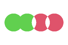
For example, the following code draws a group, using the
"xor" compositing operator, where both
the src and dst consist of
two overlapping circles. The src circles
are both filled red and the dst circles
are both filled green.
The circles are positioned in this example so that
drawing proceeds from
left to right across the image.
The left green circle is drawn
first and then the right green circle is drawn on top using
the default "over" operator. The compositing operator
is then set to "xor" and the left red circle is drawn.
This results in a gap where the right green circle and the
left red circle overlap. Finally, the right red circle
is drawn. The "xor" operator is still in effect, so the
result is a gap where the left red circle and the right
red circle overlap.
src <- circleGrob(3:4/5, r=.2, gp=gpar(col=NA, fill=2))
dst <- circleGrob(1:2/5, r=.2, gp=gpar(col=NA, fill=3))
grid.group(src, "xor", dst)
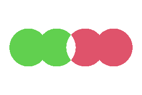
The following code shows how we can isolate src
so that the two red circles are combined using the default
"over" operator before that result is then combined with
dst using the "xor" operator. This is precisely what
groups allow us to do. The result is only a gap where
src and dst overlap.
grid.group(groupGrob(src), "xor", dst)
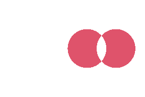
The following code demonstrates that the op
operator is in effect even when dst is NULL.
Here we only draw a src, but it consists of
two overlapping circles, and the operator is "xor", so
the second circle is "xor"ed with the first circle.
grid.group(src, "xor")
The User API Section described how groups can be used to produce a different result when a mask is in effect. This section looks at other combinations of groups with patterns and masks.
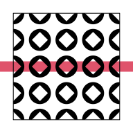
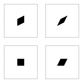
The following code shows that a group can be the basis for a tiling pattern. We create a group that combines a rotated rectangle on a black circle using the "dest.out" operator (creating a diamond-shaped hole in the circle) and then use that group as a repeating pattern to fill a rectangle. A red horizontal line is drawn first to illustrate that the diamond shape is a hole in the circle, not a white diamond drawn on top of the circle.
gp <- groupGrob(rectGrob(width=.1, height=.1, gp=gpar(fill="black"),
                         vp=viewport(angle=45)),
                "dest.out",
                circleGrob(r=.1, gp=gpar(fill="black")))
pat <- pattern(gp, width=.25, height=.25, extend="repeat")
grid.segments(y0=.5, y1=.5, gp=gpar(col=2, lwd=15))
grid.rect(width=.8, height=.8, gp=gpar(fill=pat))
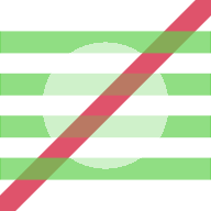
The following code shows that a group can also be the basis for a mask. We create a group that combines a solid disk, a semitransparent circle, and a semitransparent rectangle, where the circle is more translucent than the rectangle. The group consists of the circle "over" a sub-group that consists of the disk "dest.out" the rectangle; in the sub-group, the disk creates a hole in the rectangle. The overal group consists of the rectangle except where the circle and the rectangle overlap, in which case the circle is drawn. This produces a semitransparent rectangle with a more translucent circle in its centre. We push a viewport with this group as the mask and draw a series of thick, horizontal, green lines with the result that the semitransparency of the mask is transferred to the lines. A red diagonal line is drawn first to illustrate that the green lines are semitransparent.
solid <- circleGrob(r=.3, gp=gpar(col=NA, fill="black"))
circle <- circleGrob(r=.3, gp=gpar(col=NA, fill=rgb(0,0,0,.3)))
rectangle <- rectGrob(gp=gpar(fill=rgb(0,0,0,.7)))
gp <- groupGrob(circle,
                "over",
                groupGrob(solid, "dest.out", rectangle))
grid.segments(gp=gpar(col=2, lwd=20))
pushViewport(viewport(mask=gp))
grid.segments(0, 1:4/5, 1, 1:4/5, gp=gpar(col=3, lwd=20))
As hinted at in the User API Section, group affine
transformations work quite differently to the "normal"
'grid' transformations - the transformations that occur as a result of
pushing 'grid' viewports and
using the unit() function to associate locations
and dimensions with different coordinate systems within the
current viewport. The following code and output attempts to
contrast the behaviour of groups with normal 'grid' behaviour.
We begin by defining some 'grid' grobs:
a rectangle that has an absolute width (specified in inches);
a rectangle that has a relative width (specified in
"npc" coordinates);
and a text label.
We also define two 'grid' gTree objects, each of which
contains one of the rectangles plus the text label.
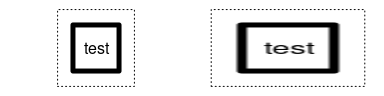
r1 <- rectGrob(width=unit(.48, "in"), height=.6, gp=gpar(lwd=5))
r2 <- rectGrob(width=unit(.6, "npc"), height=.6, gp=gpar(lwd=5))
t <- textGrob("test")
gt1 <- gTree(children=gList(r1, t))
gt2 <- gTree(children=gList(r2, t))
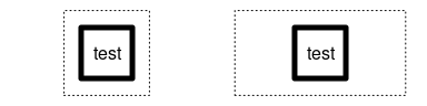
The following code draws the first gTree normally,
once in a square viewport and once in a wider
viewport (as indicated by the dotted lines).
The size of the rectangle does not change
because its width is absolute. In more detail, the
width of the rectangle, unit(.48, "in"),
is evaluated when the rectangle is drawn and the result
is the same in both viewports because .48in is the
same regardless of the size of the viewport.
The text remains the same because it is drawn in the centre of the viewport and its size is absolute (12pt).
grid.newpage()
pushViewport(viewport(x=1/4, width=.2, height=.8))
grid.rect(gp=gpar(lty="dotted"))
grid.draw(gt1)
popViewport()
pushViewport(viewport(x=3/4, width=.4, height=.8))
grid.rect(gp=gpar(lty="dotted"))
grid.draw(gt1)
popViewport()
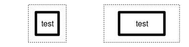
The next code draws the second gTree normally, again in both a square viewport and a wider viewport. This time, because the width of the rectangle is relative, the rectangle is wider when it is drawn in the wider viewport; .6npc means 60% of the width of the parent viewport. The text is unchanged because its height (and width) are absolute.
pushViewport(viewport(x=1/4, width=.2, height=.8))
grid.rect(gp=gpar(lty="dotted"))
grid.draw(gt2)
popViewport()
pushViewport(viewport(x=3/4, width=.4, height=.8))
grid.rect(gp=gpar(lty="dotted"))
grid.draw(gt2)
popViewport()
The next code demonstrates the different behaviour of group
affine transformations.
In the square viewport, we define a group based on the first
gTree and draw (use) that group. This produces the same
output as normal 'grid' drawing.
In the wider rectangle, when we draw (reuse) the group,
the difference between the square viewport (where the group
was defined) and the wider viewport (where the group is
being used) induces a transformation. The transformation
includes a translation, because the wider viewport is to the
right of the square viewport, and a scaling, because the
wider viewport is wider than the square viewport.
However, this transformation applies to everything that we
draw: the rectangle is not only wider, but the lines
that are used to draw the vertical sides of the rectangle
are
pushViewport(viewport(x=1/4, width=.2, height=.8))
grid.rect(gp=gpar(lty="dotted"))
grid.define(gt1, name="group")
grid.use("group")
popViewport()
pushViewport(viewport(x=3/4, width=.4, height=.8))
grid.rect(gp=gpar(lty="dotted"))
grid.use("group")
popViewport()
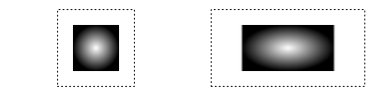
The "normal" 'grid' behaviour is useful because we do not, for example, usually want text to be distorted. However, the affine transformations that we get by reusing groups can be harnessed to achieve some useful effects. For example, the following code demonstrates that we can use affine transformations to fill a non-square region with a radial gradient. The main idea is that we define the gradient within a square region, but use it in a rectangular region. The result on the right is the image that we want to achieve and the result on the left is just for illustrative purposes. We do not need to use the gradient in the square region; we just need to define the gradient in the square region.
grad <- radialGradient(c("white", "black"))
r <- rectGrob(width=.6, height=.6, gp=gpar(col=NA, fill=grad))
pushViewport(viewport(x=1/4, width=.2, height=.8))
grid.rect(gp=gpar(lty="dotted"))
grid.define(r, name="rect")
grid.use("rect")
popViewport()
pushViewport(viewport(x=3/4, width=.4, height=.8))
grid.rect(gp=gpar(lty="dotted"))
grid.use("rect")
popViewport()
Another issue that requires more explanation is the precise transformation that is induced by defining a group within one viewport and using the group within a different viewport. There are three aspects to consider: differences in viewport location, which induce a translation; differences in viewport size, which induce a scaling; and differences in viewport angle, which induce a rotation.
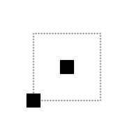
The first point is that the translation induced by a viewport is based on the (x, y) location of the viewport. In all previous examples, we have used viewports that are centred on their (x, y) location, but that does not have to be the case. For example, in the code below, we define a black rectangle within a viewport that is centred on (.5, .5) (and we draw the rectangle to show where it would appear if it was used within the same viewport), but we then use the black rectangle within a viewport that is bottom-left justified at (.25, .25). Both viewports have a width and height of .5, so they occupy the same region within the image (indicated by the dotted line), but the difference in the (x, y) location of the viewports (centre of the dotted region versus bottom-left of the dotted region) induces a translation and the reuse of the black rectangle draws it at a different location (the bottom-left of the dotted region, which is where it is used, instead of the centre of the dotted region, which is where it was defined).
pushViewport(viewport(width=.5, height=.5))
grid.rect(gp=gpar(lty="dotted"))
grid.define(rectGrob(width=.2, height=.2, gp=gpar(fill="black")),
            name="r")
grid.use("r")
popViewport()
pushViewport(viewport(x=.25, y=.25, width=.5, height=.5,
                      just=c("left", "bottom")))
grid.use("r")
popViewport()
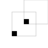
The translation is induced this way because it makes it easier to position the reuse of a group relative to a specific location using a justification other than "centred". For example, the following code defines a black rectangle bottom-left justified at the bottom-left corner of a viewport that is bottom-left justified at (.5, .5). We then use the rectangle within a viewport that is bottom-left justified at (.25, .25). This provides accurate control of the placement of the bottom-left corner of the group. (The previous example provided accurate control of the placement of the centre of the group.)
pushViewport(viewport(.5, .5, just=c("left", "bottom"),
                      width=.5, height=.5))
grid.rect(gp=gpar(lty="dotted", fill=NA))
grid.define(rectGrob(0, 0, just=c("left", "bottom"),
                     width=.2, height=.2,
                     gp=gpar(fill="black")),
            name="r")
grid.use("r")
popViewport()
pushViewport(viewport(.25, .25, just=c("left", "bottom"),
                      width=.5, height=.5))
grid.rect(gp=gpar(lty="dotted", fill=NA))
grid.use("r")
popViewport()
The scaling and rotation transformations that are induced by differences in viewport size and angle are more straightforward, though it is worth pointing out that the differences in viewport size are differences in absolute size (in inches) and take no notice of the viewport scales.
It is also worth pointing out that the overall transformation that is induced by differences between viewports may involve a combination of translation, scaling, and/or rotation. The overall transformation is calculated by a translation from the original location (where the group was defined) to the origin (0, 0), followed by scaling, rotation, and then translation to the new location (where the group is to be used).
Because the transformation is only dependent on differences in
viewport location, size, and angle, it is not possible to
induce the full range of affine transformations.
For example, although we can distort a group, by applying
a different amount of scaling in the x-direction compared to
the y-direction, we cannot induce a shear transformation.
However, the transform argument to the
grid.use() function allows us to customise
the transformation that will occur.
The transform argument must be a function that
takes two arguments, group and device,
and returns a 3x3 affine transformation matrix.
In theory, we can provide
any function that returns a 3x3 matrix
(as long as the last column contains 0, 0, and 1),
but generating a
meaningful transformation matrix requires a good understanding
of affine transformations and 'grid' internals.
Several predefined
functions are provided to make it easier to generate a custom
transformation.
The default value of transform is the
viewportTransform() function. This function
automatically generates a transformation matrix based on the
difference between the viewport where the group was defined
and the viewport where the group is being used.
A simple customisation that we can perform is to use the shear
argument to viewportTransform().
This allows us to specify a 3x3 matrix that describes a shear transform.
A shear transformation is described by two parameters: the amount of shear
in the x-direction and the amount of shear in the y-direction.
The groupShear() function is provided to generate a matrix
from just two values. For example, the following code
defines a group in a viewport in the bottom-left corner of the image
then reuses it in three viewports in
each of the other three corners of the image.
The different locations of the viewports induce a translation,
but we also specify a custom transform in each reuse
that is a function that adds a shear to the
default viewport transformation. This results in different
shear transformations of the rectangle (in addition to the
default translations). Notice that the custom transform
function uses an ellipsis argument (...) to pass through the
group and device arguments.
pushViewport(viewport(.25, .25, width=.4, height=.4))
grid.rect(gp=gpar(lty="dotted"))
grid.define(rectGrob(width=.2, height=.2, gp=gpar(fill="black")),
            name="r")
grid.use("r")
popViewport()
pushViewport(viewport(.75, .25, width=.4, height=.4))
grid.rect(gp=gpar(lty="dotted"))
grid.use("r",
         trans=function(...) viewportTransform(...,
                                               shear=groupShear(sx=.5, sy=0)))
popViewport()
pushViewport(viewport(.25, .75, width=.4, height=.4))
grid.rect(gp=gpar(lty="dotted"))
grid.use("r",
         trans=function(...) viewportTransform(...,
                                               shear=groupShear(sx=0, sy=.5)))
popViewport()
pushViewport(viewport(.75, .75, width=.4, height=.4))
grid.rect(gp=gpar(lty="dotted"))
grid.use("r",
         trans=function(...) viewportTransform(...,
                                               shear=groupShear(sx=.5, sy=.5)))
popViewport()
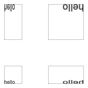
Another transformation that cannot be induced by differences between
viewports is an inversion of the x-scaling or y-scaling.
The viewportTransform() function provides
a flip argument to allow this sort of transformation
to be specified.
The following code demonstrates this argument by first defining
a group based on
a piece of text in the bottom-left of a bottom-left justified
viewport (in the bottom-left corner of the image).
The group is then used in a taller viewport that is top-left
justified, with flipY=TRUE. The resulting text
is twice as high and inverted vertically.
The group is used in two further viewports to show
inversion of the x-scaling (bottom-right) and inversion of
both scales (top-right).
pushViewport(viewport(.05, .05, just=c("left", "bottom"),
                      width=.2, height=.2))
grid.rect(gp=gpar(lty="dotted"))
grid.define(textGrob("hello", 0, 0, just=c("left", "bottom")),
            name="t")
grid.use("t")
popViewport()
pushViewport(viewport(.05, .95, just=c("left", "top"),
                      width=.2, height=.4))
grid.rect(gp=gpar(lty="dotted"))
grid.use("t",
         trans=function(...) viewportTransform(...,
                                               flip=groupFlip(flipY=TRUE)))
popViewport()
pushViewport(viewport(.95, .05, just=c("right", "bottom"),
                      width=.4, height=.2))
grid.rect(gp=gpar(lty="dotted"))
grid.use("t",
         trans=function(...) viewportTransform(...,
                                               flip=groupFlip(flipX=TRUE)))
popViewport()
pushViewport(viewport(.95, .95, just=c("right", "top"),
                      width=.4, height=.4))
grid.rect(gp=gpar(lty="dotted"))
grid.use("t",
         trans=function(...) viewportTransform(...,
                                               flip=groupFlip(flipX=TRUE,
                                                              flipY=TRUE)))
popViewport()
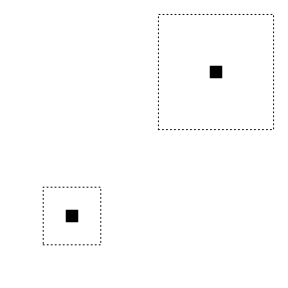
It is also possible to specify a custom transformation
in order to simplify the transformation that is induced
by differences between viewports.
For example, we can ensure that only translations occur
and any differences in viewport size are ignored.
The following code demonstrates this idea by first
defining a group based on a rectangle in a small viewport
(bottom-left).
The group is then used in a larger viewport, but with
viewportTranslate() as the transformation function.
The resulting rectangle is the same size as the original
rectangle because viewportTranslate() only
takes any notice of differences in location between
viewports; it ignores differences in size.
pushViewport(viewport(.25, .25, width=.2, height=.2))
grid.rect(gp=gpar(lty="dotted"))
grid.define(rectGrob(width=.2, height=.2, gp=gpar(fill="black")),
            name="r")
grid.use("r")
popViewport()
pushViewport(viewport(.75, .75, width=.4, height=.4))
grid.rect(gp=gpar(lty="dotted"))
grid.use("r",
         trans=viewportTranslate)
popViewport()
It is also possible to transform a group without having to
use it in a different viewport; we can just provide a
transform argument to grid.use().
However, this sort of "raw" transformation takes place
in the device coordinate system, which can make it difficult
to determine the correct transformation.
For example, the device origin (0, 0) is top-left for
a Cairo device on screen and bottom-right is likely to be
several hundred pixels in both dimensions.
The following code demonstrates how this might produce
initially confusing results from naive code.
We specify a transform function that
calls groupRotate to generate an matrix
that generates an anti-clockwise rotation of 30 degrees.
However, the result is an anti-clockwise rotation of 30 degrees
around the origin, where the origin is the top-left
of the image.
grid.define(rectGrob(width=.4, height=.4,
                     gp=gpar(fill=rgb(0,0,0,.5))),
            name="r")
grid.use("r")
grid.use("r", transform=function(...) groupRotate(30))

If we want to rotate the rectangle (in place), we need to
translate to the device origin, rotate, and translate back.
And in order to translate, we need to know the position of
the rectangle on the device. The following code
uses deviceLoc() to determine the correct
location on the device and defines a transformation function
that correctly rotates the rectangle.
grid.define(rectGrob(width=.4, height=.4,
                     gp=gpar(fill=rgb(0,0,0,.5))),
            name="r")
grid.use("r")
loc <- deviceLoc(unit(.5, "npc"), unit(.5, "npc"), device=TRUE)
trans <- function(...) {
    groupTranslate(-loc$x, -loc$y) %*%
    groupRotate(30) %*%
    groupTranslate(loc$x, loc$y)
}
grid.use("r", transform=trans)

To further complicate matters, that transformation is only correct
for when the transformation is called with device=TRUE
(the custom transformation function above just ignores the
device argument).
This demonstrates why it will usually be easier to specify the transformation through a change in viewport, as shown by the code below.
grid.define(rectGrob(width=.4, height=.4,
                     gp=gpar(fill=rgb(0,0,0,.5))),
            name="r")
grid.use("r")
pushViewport(viewport(angle=30))
grid.use("r")

vp argument
All of the functions grid.group(),
grid.define(), and grid.use()
have a vp argument. This allows us to
specify a viewport that will be pushed before the group
is drawn (or defined or used) and then navigated up out of
afterwards.
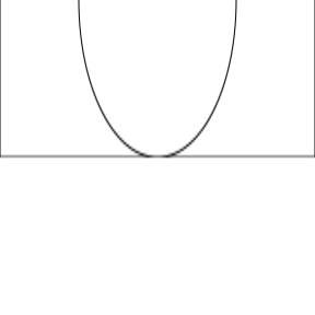
For grid.group(), this is straightforward,
the viewport is pushed, the group is defined and used,
and then we come up out of the viewport. For example,
the code below draws a group within a temporary viewport
in the bottom half of the image.
vp <- viewport(y=0, height=.5, just="bottom")
grid.group(grobTree(rectGrob(), circleGrob()),
           vp=vp)

Normally, when we use grid.define() and
grid.use(), if we call them within the same
viewport, we will draw the untransformed group.
However, if we specify a viewport via the vp
argument in the call to
grid.define(), but not in grid.use(),
the group definition will occur in a different viewport than the
group use and the group will be transformed, as shown below
(notice that the viewport for the group use is not only
taller, but has a different x/y location compared to the
viewport for the group definition because the viewport for
the group definition was bottom-justified at y=0 while the viewport
for the group use is centred at y=.5).
grid.define(grobTree(rectGrob(), circleGrob()),
            vp=vp,
            name="groupvp")
grid.use("groupvp")
We can of course get the untransformed group by specifying the
same viewport via vp in the grid.use()
call, so that the group definition and the group use occur
within the same viewport, as shown below.
grid.define(grobTree(rectGrob(), circleGrob()),
            vp=vp,
            name="groupvp")
grid.use("groupvp",
         vp=vp)
This section returns to the more complex example from the Introduction Section. Now that we have seen how the new graphics features work, we can explain how to produce this plot. This example also demonstrates that groups can be based on any 'grid' grob, including a grob that represents an entire 'ggplot2' plot.
The plot that we will work with is defined with the following code.
library(ggplot2)
gg <- ggplot(mtcars) +
    geom_point(aes(disp, mpg)) +
    theme_bw() +
    theme(panel.background=element_rect(color=NA, fill="transparent"),
          plot.background=element_rect(color=NA, fill="transparent"))
The code below begins by pushing a viewport that is bottom-left justified at the bottom-left corner of the image (and only occupies 60% of the width of the image). We then capture the 'grid' gTree that would be drawn by this plot (and make all lines double thickness). We also define a group based on that gTree. Next, we define a transformation function that will add a shear in the x-direction to the default viewport transformation. We push a new viewport that is much shorter than the first viewport. This induces a scaling in the y-direction. This viewport also enforces a semitransparent mask. We use the group in this new viewport, specifying our custom transformation, which produces a semitransparent, vertically squashed, and horizontally skewed version of the plot. Finally, we pop the second viewport and draw the original group over the top of its squashed and skewed "shadow".
pushViewport(viewport(x=0, y=0, width=.6,
                      just=c("left", "bottom")))
g <- editGrob(grid.grabExpr(plot(gg), gp=gpar(lex=2)))
grid.define(g, name="g")
trans <- function(...) {
    viewportTransform(..., shear=groupShear(2, 0))
}
pushViewport(viewport(x=0, y=0, height=1/4, just=c("left", "bottom"),
                      mask=rectGrob(width=2,
                                    gp=gpar(col=NA, fill=rgb(0,0,0,.7)))))
grid.use("g", transform=trans)
popViewport()
grid.draw(g)
In simple situations, groups behave very much like a standard 'grid' gTree. A group consists of one or more grobs and when we draw the group we just draw that collection of grobs. However, previous sections have demonstrated that, by specifying different compositing operators, or by defining a group in one viewport and using it in another, we can get behaviour that deviates from standard gTrees. This section demonstrates that, even in simple situations, when a group produces the same graphical output as an equivalent gTree, there are some things that still work differently.
In order to demonstrate the differences, we will work with a red rectangle grob and a green circle grob.
r <- rectGrob(gp=gpar(col=NA, fill=2, lwd=3), name="r")
c <- circleGrob(r=.4, gp=gpar(col=NA, fill=3, lwd=3), name="c")
The following code creates a gTree with the rectangle and the circle
as its children. We draw the gTree and then use grid.ls()
to list the grobs in our image.
The result shows that we have a gTree with a rectangle (r)
and a circle (c) as its children.
gt <- gTree(children=gList(r, c), name="gTree")
grid.draw(gt)
grid.ls()
  gTree
    r
    c
We can now use the grid.edit() function to modify the
gTree or its children. In the code below we shrink the width
of the rectangle.
grid.edit("r", width=unit(.5, "npc"))
The following code creates a group equivalent of the gTree.
In this group, the src is the circle and the
dst is the rectangle (and the default operator
is "over"), so when we draw the group, we get the same result
as the gTree.
grid.group(src=c, dst=r, name="group")

However, if we list the grobs in the image, all we can see is the group grob.
grid.ls()
group
This demonstrates that the src and dst
of a group are not the same as the children of a gTree.
A gTree draws its children, but a group is defined by
its children.
This also means that we cannot directly access the grobs that
define a group with a single gPath (like we can with the children
of a gTree).
However, it is still possible to modify the definition of
a group, as shown in the code below.
grid.edit("group", dst=editGrob(r, width=unit(.5, "npc")))

grid.edit("group", op="xor")
This section deals with more advanced 'grid' concepts and assumes a strong familiarity with 'grid'. It builds on the ideas of listing and editing individual grobs within an image, but deals with more complex scenarios than the previous section.
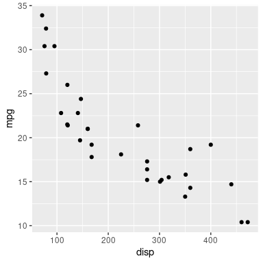
It is possible to create 'grid' grobs that generate their content when they are drawn. An example is the grob that a 'ggplot2' plot creates. For example, the following code defines a 'ggplot2' plot, draws it, and lists the grob that has been created.
g <- ggplot(mtcars) + geom_point(aes(disp, mpg))
plot(g)

grid.ls()
layout
The listing only shows a single grob with no children. This is a "gtable" grob that contains all of the information necessary to draw the 'ggplot2' plot, but it has not created all of the individual text and rectangle grobs for the plot yet; it does that every time it gets drawn.
If we want to access the individual text and rectangle grobs for the plot, we have to "force" the "gtable" grob. The following code does this and shows that there are now lots of individual grobs.
grid.force()
grid.ls()
  layout
    background.1-9-12-1
      plot.background..rect.492
    panel.7-5-7-5
      panel-1.gTree.472
        grill.gTree.470
          panel.background..rect.461
          panel.grid.minor.y..polyline.463
          panel.grid.minor.x..polyline.465
          panel.grid.major.y..polyline.467
          panel.grid.major.x..polyline.469
        NULL
        geom_point.points.457
        NULL
        panel.border..zeroGrob.458
    spacer.8-6-8-6
      NULL
    spacer.8-4-8-4
      NULL
    spacer.6-6-6-6
      NULL
    spacer.6-4-6-4
      NULL
    axis-t.6-5-6-5
      NULL
    axis-l.7-4-7-4
      GRID.absoluteGrob.480
        NULL
        axis
          axis.1-1-1-1
            GRID.titleGrob.478
              GRID.text.477
          axis.1-2-1-2
            GRID.polyline.479
    axis-r.7-6-7-6
      NULL
    axis-b.8-5-8-5
      GRID.absoluteGrob.476
        NULL
        axis
          axis.1-1-1-1
            GRID.polyline.475
          axis.2-1-2-1
            GRID.titleGrob.474
              GRID.text.473
    xlab-t.5-5-5-5
      NULL
    xlab-b.9-5-9-5
      axis.title.x.bottom..titleGrob.483
        GRID.text.481
    ylab-l.7-3-7-3
      axis.title.y.left..titleGrob.486
        GRID.text.484
    ylab-r.7-7-7-7
      NULL
    subtitle.4-5-4-5
      plot.subtitle..zeroGrob.488
    title.3-5-3-5
      plot.title..zeroGrob.487
    caption.10-5-10-5
      plot.caption..zeroGrob.490
    tag.2-2-2-2
      plot.tag..zeroGrob.489
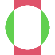
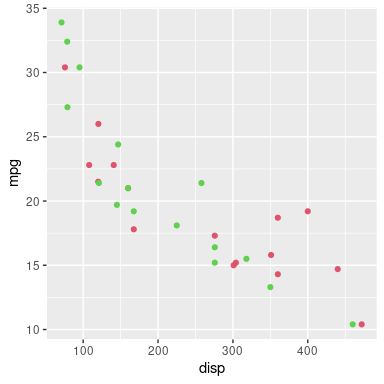
The next code modifies the individual points grob to colour the points alternating red and green
grid.edit("points", grep=TRUE, gp=gpar(col=2:3))

It is possible to create a group based on a grob that only generates its content when it is drawn. For example, the following code creates a group based on the 'ggplot2' plot from above.
ggrob <- ggplotGrob(g)
gp <- groupGrob(ggrob, name="group")
As the previous section pointed out, grid.ls()
and grid.edit() cannot see or access the src
or dst of a group grob.
For the group that we just defined, when we look at the group
src, we cannot see any of its individual grobs either;
the src is just a "gtable" grob that will generate
its individual grobs when it gets drawn.
This is illustrated in the output from grid.ls() below.
grid.ls(gp)
group
grid.ls(gp$src)
layout
In this situation it is doubly hard to access and modify the grobs within a group. However, it is still possible if we edit the grob before we use it to define a group. For example, the following code forces the 'ggplot2' plot grob and edits it before defining a group based on the edited grob. The result is a group based on the modified 'ggplot2' plot.
ggrobForced <- forceGrob(ggrob)
ggrobMod <- editGrob(ggrobForced, "points", grep=TRUE,
                     gp=gpar(col=2:3))
grid.group(ggrobMod)
A slightly more difficult scenario arises when we want to
edit the individual grobs within a group that someone else's
code has drawn. In this case, we need to access the group,
access the src grob within the group, force
that src grob, modify the forced grob, and
edit the group to replace the original src
with the new forced and modified version.
The following code demonstrates this idea,
starting with a group that is drawn from a 'ggplot2'
"gtable" grob; this represents a group that has already
been drawn based on a src grob that generates
its individual grobs only when it is drawn.
grid.group(ggrob, name="group")
gp <- grid.get("group")
src <- gp$src
srcForced <- forceGrob(src)
srcMod <- editGrob(srcForced, "points", grep=TRUE,
                   gp=gpar(col=2:3))
grid.edit("group", src=srcMod)

This section describes the impact that the changes to R will have on packages that provide a graphics device, like the 'ragg' package (Pedersen and Shemanarev, 2021).
The good news is that maintainers of R packages that implement
graphics devices do not need to do anything in response
to these changes. Graphics device packages will need to be reinstalled
for R version 4.2.0, but they do not need to be updated.
The graphics engine will only make calls to the graphics device
to define or use groups if the graphics device deviceVersion
is set to 15 (R_GE_group) or higher. Of course, if
the graphics device has a lower deviceVersion,
R code that defines or uses groups will have no effect.
A device can be updated, by setting
dev->deviceVersion to 15
(R_GE_groups), but it does not have to offer support
for the new features.
As an example of the (minimal) changes necessary to update a device
(without support for any of the new group features),
the following diff output
shows the changes made to the postscript()
device.
@@ -3033,6 +3033,14 @@
+static SEXP     PS_defineGroup(SEXP source, int op, SEXP destination,
+                               pDevDesc dd);
+static void     PS_useGroup(SEXP ref, SEXP trans, pDevDesc dd);
+static void     PS_releaseGroup(SEXP ref, pDevDesc dd);

@@ -3495,11 +3503,17 @@
+    dd->defineGroup     = PS_defineGroup;
+    dd->useGroup        = PS_useGroup;
+    dd->releaseGroup    = PS_releaseGroup;

-    dd->deviceVersion = R_GE_definitions;
+    dd->deviceVersion = R_GE_group;

@@ -4535,8 +4549,22 @@
+static SEXP PS_defineGroup(SEXP source, int op, SEXP destination, pDevDesc dd) {
+    return R_NilValue;
+}

+static void PS_useGroup(SEXP ref, SEXP trans, pDevDesc dd) {}

+static void PS_releaseGroup(SEXP ref, pDevDesc dd) {}
This section provides information about what to do if a graphics device package wishes to provide support for the new group features.
The dev->deviceVersion must be set to 15
(R_GE_groups) or higher.
A device must implement the new dev->defineGroup
function. The first and third arguments to this function
(source and destination)
are R function objects,
with the destination potentially NULL.
If destination is not NULL,
the device should evaluate the destination function.
As with
clipping paths and masks
(Murrell, 2020b),
this will generate further calls to the device to draw shapes,
which the device should capture to define the "destination"
(rather than drawing immediately).
For example, the Cairo devices perform the drawing within a
cairo_push_group and cairo_pop_group;
the pdf() device records the drawing within
temporary strings.
The device should next set the compositing operator based on
the second argument to dev->defineGroup, called
op. This should happen
regardless of whether destination
is NULL or not. The C API provides
R_GE_compositeClear,
R_GE_compositeSource,
R_GE_compositeOver, etc to switch on.
The device should then evaluate the source function
and capture the resulting drawing as the "source".
This combination of destination (maybe) combined with
source using the given compositing operator defines the group.
The device should return a reference to the resulting group
definition. This reference can be any R object; it only has to make
sense to the device.
The device must enforce the current graphical parameter settings when creating the group definition, so that these are fixed for when the group is used.
A device must also implement the new dev->useGroup.
The first argument is a reference to a group definition
(taken from the return value of a call to dev->defineGroup).
The second argument is a 3x3 R matrix object that specifies
an affine transformation.
The device should apply the transformation and
combine the group with any previous drawing using
the normal "over" operator.
Finally, the device should implement dev->releaseGroup.
The first argument to this function is a reference to an existing
group. This allows the device to release resources associated
with a group.
Support for these new features has been implemented for the
pdf() device, the
quartz() device (from R 4.3.0),
and the devices that are based on Cairo
graphics, so the code for those devices demonstrates some
possible approaches to implementation.
In both of these cases, the infrastructure that was previously
added to support
fill patterns, clipping paths, and masks has been reused
(Murrell, 2020b).
For the pdf() device, defineGroup
creates temporary strings to
capture PDF code during the evaluation of the source
and destination functions. These, along with the
op are used to define the content stream of an
XObject that can be referenced elsewhere in the PDF document.
An integer index is returned as the result.
The useGroup implementation sets up the
appropriate transformation matrix and performs a
Do operation with a reference to the relevant
XObject.
The releaseGroup implementation does nothing.
For Cairo devices, defineGroup uses
cairo_push_group() to capture Cairo drawing
operations as a separate image. Any drawing
during the evaluation of source and
destination is captured to that image, with the op
compositing operator set between evaluating destination and
source.
The image is held in memory until the group is released.
Again, an integer index to the group is returned as the result.
The useGroup implementation sets up an
appropriate transformation matrix and then uses the relevant
group image to paint the group on the main image.
The releaseGroup implementation releases the
group image from memory.
The addition of groups to the R graphics engine significantly extends the range of graphical effects that can be achieved with R code. As mentioned in the introduction, the primary motivation for these changes is to provide access to more sophisticated graphical features in graphics formats like PDF and graphics systems like Cairo, so that more can be achieved purely in R code rather than having to fine-tune images manually outside of R.
The most important limitation to acknowledge is the fact that
these new features are only currently supported on a subset
of the core graphics devices: the pdf() device
and the devices based on Cairo graphics (e.g.,
png(type="cairo"),
cairo_pdf() and svg()).
Furthermore, the Porter-Duff compositing operators are only
supported on the Cairo devices.
The 'ragg' package is adding support for the previous set of graphics features (gradients, patterns, clipping paths, and masks), so there is hope that the 'ragg' package will also be able to support this new set of features as well in the future.
Although the user interface for the new features is limited
to the low-level 'grid' graphics system, any high-level graphics system
that is built on 'grid', like 'ggplot2', can also make use
of the new features, either by post-hoc editing with functions like
grid.edit(), or, in the case of 'ggplot2', by adding layers
with the
'gggrid' package (Murrell, 2021b).
Thanks to the 'gridGraphics' package (Murrell and Wen, 2020),
it is also possible to work with plots from the 'graphics' package
by converting them to 'grid' equivalents and then using post-hoc editing.
The addition of these new features broadens the range of graphical output that is possible with R graphics. This narrows the gap between R graphics and some other graphics systems like PGF/TikZ (Tantau, 2021). For example, the ability to apply affine transformations is similar to the "canvas" coordinate system within PGF. On one hand this allows users to generate graphical images within a single system rather than having to mix systems in order to get specific features. On the other hand, this improves our ability to exchange output between systems without losing features. For example, the 'dvir' package (Murrell, 2021a; Murrell, 2020a) should be able to correctly import and render a wider range of TikZ output.
Similarly, the packages 'grImport' (Murrell, 2009) and 'grImport2' (Potter and Murrell, 2019) which import PostScript and SVG images to R should be able to import and correctly reproduce a wider range of external images.
Several other packages provide ways to expand the range of graphical output in R, many of them as extensions to the 'ggplot2' system. For example, 'ggpattern' (FC, 2020) provides functions for generating pattern fills and 'ggtext' (Wilke, 2020) provides more complex text formatting. The 'ggfx' package (Pedersen, 2021) provides, at a raster level, compositing operators, plus a whole range of other filters. There is also some overlap with the 'gridGeometry' package (Murrell, 2019), which allows shapes to be combined, e.g., with an "xor" operator, before rendering the result. In all of these cases, the additional features within the R graphics engine should make it easier for those packages to do their work (at least on some graphics devices). Because they do not rely on graphics device support, the enduring usefulness of these packages will be their ability to work across a wider range of R graphic devices. On the other hand, some of the new features, for example affine transformations, are not currently available any other way in R graphics.
Thanks to the CRAN group, particularly Brian Ripley, for assistance with testing and coordinating the merge of these changes into R.
Thanks to Trevor Davis for early testing that lead to
important fixes in the handling of transformations
induced by grid.use().
The examples and discussion in this report relate to R version 4.2.0. The examples involving compositing operators now relate to R version 4.3.0.
This report was generated within a Docker container (see Resources section below).
Murrell, P. (2021). "Groups, Compositing Operators, and Affine Transformations in R Graphics" Technical Report 2021-02, Version 3, Department of Statistics, The University of Auckland. Version 1. [ bib | DOI | http ]
This document
by Paul
Murrell is licensed under a Creative
Commons Attribution 4.0 International License.