 http://orcid.org/0000-0002-3224-8858
by Paul Murrell
 http://orcid.org/0000-0002-3224-8858
Version 1: Tuesday 16 November 2021

This document
by Paul
Murrell is licensed under a Creative
Commons Attribution 4.0 International License.
This document describes an expansion of the R graphics engine to support stroking and filling paths.
These features are available in the development version of R (to become 4.2.0).
R users wanting to try out the new graphics features should start with the User API Section, which provides a quick introduction to the new R-level interface.
Maintainers of R packages that provide R graphics devices should read the Device API Section, which provides a description of the required changes to R graphics devices.
These new graphics features have not (yet) been implemented for
all of the graphics devices provided by the 'grDevices'
package. Devices that do support the new features are the
pdf() graphics device and Cairo graphics devices:
x11(type="cairo"), cairo_pdf(),
cairo_ps(), png(type="cairo"),
jpeg(type="cairo"), tiff(type="cairo"),
and svg().
The remainder of the graphics
devices in 'grDevices' will run, but will (silently) not produce
the correct output. Graphics devices from other R packages should
be reinstalled and will not produce the correct output until
(or unless)
the package maintainer adds support.
Changes to the graphics engine in R 4.1.0 added support for
gradient and pattern fills, clipping paths, and masks
(Murrell, 2020).
One way to think of those changes is that they
create an R interface to some of the more advanced graphical features
of specific R graphics devices; graphics devices that are based on
sophisticated graphics systems, like the pdf() device
that is based on the Adobe Portable Document Format
(Adobe Systems Incorporated, 2001) and the graphics
devices based on the Cairo graphics library (Packard et al., 2021).
This document describes another step along that path, by adding
an R interface to generate "paths" from a collection of graphical objects.
As with the group features that have been recently added to R graphics (Murrell, 2021), the main motivation behind adding the new path features is to increase the range of graphical output that can be produced entirely with R code, so that users do not have to resort to manual tweaks with software like Adobe Illustrator. As a consequence, the examples in this report involve only basic shapes that demonstrate the fundamental concepts. There are no obvious connections to traditional data visualisation, though of course the possibility of future connections arising cannot be entirely ruled out.
R graphics follows a very simple graphics model: it only draws one shape at a time. For example, the following code draws a circle and then a rectangle. Both shapes have an opaque border, but a semitransparent fill, which allows us to see that the rectangle, which is drawn second, is drawn on top of the circle.
library(grid)
grid.circle(.6, .6, r=.2,
            gp=gpar(col=4, lwd=5, fill=adjustcolor(4, alpha=.5)))
grid.rect(.4, .4, width=.4, height=.4,
          gp=gpar(col=2, lwd=5, fill=adjustcolor(2, alpha=.5)))

R graphics output is sent to a graphics device either to draw
to the screen, or to record the drawing in a file. For example,
the postscript() device records drawing
in a PostScript file.
The simplicity of R graphics means that R graphics devices are only asked to
draw one shape at a time, e.g., draw a circle then
draw a rectangle.
For example, the PostScript to draw a circle and a rectangle could look like
the following. The important part of the code is the clear separation
into two shapes, each starting with a
newpath and ending with a fill
(to fill the shape).
  %%BoundingBox: 0 0 200 200

  newpath
  120 120 40 360 0 arcn
  .13 .59 .90 setrgbcolor
  fill

  newpath
   40  40 moveto
   40 120 lineto
  120 120 lineto
  120  40 lineto
  closepath
  .87 .33 .42 setrgbcolor
  fill

  showpage

However, many graphics devices support a more sophisticated drawing
model based on paths. In this model, a single path can be
constructed from more than one shape. For example, the PostScript
code below draws the same two shapes as before, but draws them
within a single path (and then fills that single path). In this code,
we can see only one newpath and only one fill.
  %%BoundingBox: 0 0 200 200

  newpath
  120 120 40 360 0 arcn
   40  40 moveto
   40 120 lineto
  120 120 lineto
  120  40 lineto
  closepath
  .87 .33 .42 setrgbcolor
  fill

  showpage

The result in this case is a filled area that is just the union of the
two individual shapes, but we can get more interesting results by
controlling how the "inside" of the path is interpreted. For example,
the following PostScript code creates exactly the same
single path from the two shapes, but this time runs eofill
(rather than fill). That changes to an "even-odd" fill rule
(from the default "non-zero winding" rule), so the overlap
between the two shapes within the path is now "outside" the overall
path and we get a shape with a hole in it.
  %%BoundingBox: 0 0 200 200

  newpath
  120 120 40 360 0 arcn
   40  40 moveto
   40 120 lineto
  120 120 lineto
  120  40 lineto
  closepath
  .87 .33 .42 setrgbcolor
  eofill

  showpage

The changes described in this report allow us to draw these more sophisticated paths in R graphics. As a simple demonstration, the following code defines a 'grid' gTree consisting of a circle grob and a rectangle grob.
gt <- gTree(children=gList(circleGrob(.6, .6, r=.2,
                                      gp=gpar(col=4, lwd=5,
                                              fill=adjustcolor(4, alpha=.5))),
                           rectGrob(.4, .4, width=.4, height=.4,
                                    gp=gpar(col=2, lwd=5,
                                            fill=adjustcolor(2, alpha=.5)))))
If we draw this gTree normally, the circle and the rectangle are drawn as separate shapes and we get the rectangle drawn on top of the circle.
grid.draw(gt)
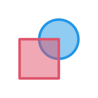
With the new changes, we can instead draw the gTree as a single path (and fill and stroke the path) with the code shown below.
grid.fillStroke(gt,
                gp=gpar(col=2, lwd=5, fill=adjustcolor(2, alpha=.5)),
                rule="evenodd")

The result is a single path based on the combination of the circle
and the rectangle and, because we specified rule="evenodd",
that path is filled and stroked using the even-odd rule
used to determine where to fill. This means that we get a hole
in the path where the two shapes overlap.
The new features for stroking and filling paths are only available via
functions in the 'grid' package (so far).
The grid.stroke() function strokes a path,
the grid.fill() function fills a path,
and the grid.fillStroke() functions fills and
strokes a path.
In all three cases, the path is defined by a 'grid' grob.
The simplest example is a single shape as in the code below.
grid.stroke(circleGrob(r=.3))
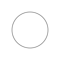
This example behaves just like normal 'grid' drawing, but already there are some important differences. For example, the following code produces exactly the same result even though it is based on a filled circle grob.
grid.stroke(circleGrob(r=.3, gp=gpar(fill="grey")))

This demonstrates an important principle of paths in R: a grob only contributes its outline to a path. The following code demonstrates that this also applies to the fill rule for a "path" grob.
First we describe a shape using the pathGrob()
function which consists of two rectangles, one nested within the
other. This includes a fill rule (winding)
that means that the
inner rectangle should be filled. This shape is drawn on the
left of the image. Next, we define a path based on this shape,
but with a different fill rule (evenodd).
When we fill the path, the
shape only contributes its outline, its fill rule
(winding) is ignored.
The fill rule for the path (evenodd) is enforced to
determine the fill region, which means that
the inner rectangle is NOT filled. This result is drawn on the right.
shape <- pathGrob(c(.2, .2, .8, .8, .4, .4, .6, .6),
                  c(.2, .8, .8, .2, .4, .6, .6, .4),
                  id=rep(1:2, each=4),
                  rule="winding",
                  gp=gpar(fill="grey"))
pushViewport(viewport(x=0, width=.5, just="left"))
grid.draw(shape)
popViewport()
pushViewport(viewport(x=.5, width=.5, just="left"))
grid.fillStroke(shape, rule="evenodd", gp=gpar(fill="grey"))
popViewport()
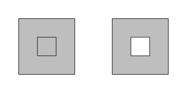
The next example demonstrates one way in which this behaviour - shapes only contribute outlines - might be useful. We use a text grob to add the outlines of text glyphs to a path and then stroke the path to produce outlined text.
grid.stroke(textGrob("outline", gp=gpar(cex=3)))
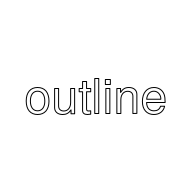
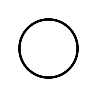
The next example shows another important point:
functions like grid.stroke() have a gp
argument that controls the graphical parameters that are
used to draw the path. In this case, a circle grob
with the default line width of 1 is used to define the path.
The grob only contributes its outline to the path; its
line width is ignored.
The grid.stroke() call specifies a line width of 5,
so the path is stroked using a thick line.
grid.stroke(circleGrob(r=.3), gp=gpar(lwd=5))
The next example is slightly more complex because it
involves a path that is based on more than one shape.
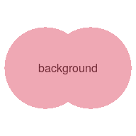
This code works with a path that is based on two overlapping
circles. We use grid.fill() this time to
fill the path.
The result is interesting because we have filled the path
with a semitransparent red (and drawn text underneath
to emphasise that we can see through the fill).
The grid.fill() function fills the "inside"
of the path, which in this case is the union of the
two circles.
grid.text("background")
grid.fill(circleGrob(1:2/3, r=.3),
          gp=gpar(fill=adjustcolor(2, alpha=.5)))
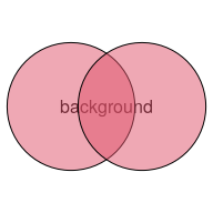
For comparison,
the following code draws the grob normally (two overlapping circles)
using a semitransparent red fill, just to emphasise how the
path-filling behaviour is different. For a start, drawing
the grob draws the circle borders (whereas grid.fill(),
will only ever fill a path), but more importantly,
drawing the grob fills each circle separately, so we get
an intersection region where the top circle partially overlaps the
bottom circle.
grid.text("background")
grid.circle(1:2/3, r=.3,
            gp=gpar(fill=adjustcolor(2, alpha=.5)))
The grid.fill() and grid.fillStroke()
functions have an additional argument, rule,
that controls the fill-rule that is used to fill the path.
The following code again fills a path based on the two overlapping circles,
but this time uses the even-odd fill rule.
This results in a filled path with a hole where the circles
overlap.
grid.text("background")
grid.fill(circleGrob(1:2/3, r=.3),
          gp=gpar(fill=adjustcolor(2, alpha=.5)),
          rule="evenodd")

Clipping paths, which were added to the R graphics system in R 4.1.0, are also based on 'grid' grobs and they produce a single path from multiple shapes just like the paths described above.
The region that output is clipped to, based on a clipping path, is the region that would be filled, if that clipping path was filled.
Unfortunately, in the original implementation of clipping paths, this distinction was not made clear and no facility was provided to specify the fill rule for a clipping path.
The new function as.path(grob, gp, rule) is designed
to help fix this problem.
This function combines a grob with graphical parameter settings
and a fill rule; it defines a path, how to fill it, and what
colours and line types to use when filling or stroking the path.
Clipping paths, as already implemented in R 4.1.0 via
viewport(clip=grob), can now also be specified
via viewport(clip=as.path(grob, gp, rule)).
This allows the fill rule for a clipping path to be specified
by the user.
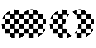
The code below demonstrates this by defining two clipping paths,
both consisting of two overlapping circles, but one using
the even-odd fill rule and one using the (default) non-zero winding rule.
circles <- circleGrob(1:2/3, r=.3)
clipPath1 <- circles
clipPath2 <- as.path(circles, rule="evenodd")
The following code pushes two viewports, one using the first clipping path (on the left) and one using the second clipping path (on the right), and fills a rectangle using a checkerboard pattern (code for the pattern not shown). We can clearly see that the clipping paths differ based on the path fill rule that is used.
pushViewport(viewport(x=0, width=.5, just="left",
                      clip=clipPath1))
grid.rect(gp=gpar(fill=pat))
popViewport()
pushViewport(viewport(x=.5, width=.5, just="left",
                      clip=clipPath2))
grid.rect(gp=gpar(fill=pat))
popViewport()
The functions grid.stroke(),
grid.fill(), and grid.fillStroke()
are all generic so the user can supply a single
argument using as.path() rather than specifying
the grobs, fill rule, and graphical parameters as separate arguments.
For example, the following two sets of code produce exactly the same
result.
grid.text("background")
grid.fill(circleGrob(1:2/3, r=.3),
          gp=gpar(fill=adjustcolor(2, alpha=.5)),
          rule="evenodd")
grid.text("background")
grid.fill(as.path(circleGrob(1:2/3, r=.3),
                  gp=gpar(fill=adjustcolor(2, alpha=.5)),
                  rule="evenodd"))
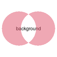
If we want to know what a clipping path is going to look like,
we can use grid.fill() on the clipping path. The
region that is filled will be the clipped region.
The good news is that maintainers of R packages that implement
graphics devices do not need to do anything in response
to these changes. Graphics device packages will need to be reinstalled
for R version 4.2.0, but they do not need to be updated.
The graphics engine will only make calls to the graphics device
to stroke or fill paths if the graphics device deviceVersion
is set to 15 (R_GE_group) or higher. Of course, if
the graphics device has a lower deviceVersion,
R code that attempts to stroke or fill paths will have no effect.
As an example of the (minimal) changes necessary to update a device
(without support for any of the new path features),
the following diff output
shows the changes made to the postscript()
device.
@@ -3033,6 +3033,14 @@
+static void     PS_stroke(SEXP path, const pGEcontext gc, pDevDesc dd);
+static void     PS_fill(SEXP path, int rule, const pGEcontext gc, pDevDesc dd);
+static void     PS_fillStroke(SEXP path, int rule, const pGEcontext gc,
+                              pDevDesc dd);

@@ -3495,11 +3503,17 @@
+    dd->stroke          = PS_stroke;
+    dd->fill            = PS_fill;
+    dd->fillStroke      = PS_fillStroke;

-    dd->deviceVersion = R_GE_definitions;
+    dd->deviceVersion = R_GE_group;

@@ -4535,8 +4549,22 @@
+static void PS_stroke(SEXP path, const pGEcontext gc, pDevDesc dd) {}
+
+static void PS_fill(SEXP path, int rule, const pGEcontext gc, pDevDesc dd) {}
+
+static void PS_fillStroke(SEXP path, int rule, const pGEcontext gc,
+                          pDevDesc dd) {}
This section provides information about what to do if a graphics device package wishes to support the new path features.
The dev->deviceVersion must be set to 15
(R_GE_groups) or higher.
A device must implement the new
dev->stroke(path, gc, dd),
dev->fill(path, rule, gc, dd), and
dev->fillStroke(path, rule, gc, dd) functions.
The path argument is an R function that the
device should evaluate to define the path.
As with clipping paths, masks, and groups,
this function will generate further calls to the device, which the device
should "capture" to define the path (rather than drawing immediately).
For dev->fill and dev->fillStroke,
the rule argument is an integer and
the device should set the fill rule based on this
(the graphics engine provides R_GE_nonZeroWindingRule
and R_GE_evenOddRule to switch on).
The device should then stroke, fill, or fill and stroke the path
(ideally, the graphics system being used will have a single
operator that performs the latter) using the current
graphical parameter settings provided in the gc argument.
The existing dev->setClipPath(path, ref, dd) API
is unchanged;
the fill rule for the clipping path function is passed in
via attr(path, "rule").
Support for these new features has been implemented for the
pdf() device and the devices that are based on Cairo
graphics, so the code for those devices demonstrates some
possible approaches to implementation.
Both Cairo and PDF devices use the "append mode" previously introduced for capturing clipping paths (Murrell, 2020) to accumulate a path before stroking or filling it.
The most important limitation to acknowledge is the fact that
these new features are only currently supported on a subset
of the core graphics devices: the pdf() device
and the devices based on Cairo graphics (e.g.,
png(type="cairo"),
cairo_pdf() and svg()).
In addition, the pdf() device
only allows a single text object within a path
(no combining text with other drawing in a path).
Other drawing is just left out of a path that already contains text
and text is left out of a path
if other drawing already exists.
This also applies to clipping paths on the pdf()device.
As with groups (Murrell, 2021)
we cannot directly see (grid.ls()) or edit
(grid.edit()) the
grob that defines a path. However, with a little extra work,
it is possible to extract the
path component of a stroke, fill, or fillStroke
grob and edit/replace that.
The 'grid' graphics system already had a "path" interface
with its grid.path() function.
The difference between that interface and this new one
is that a grid.path() can only be constructed
from a set of vertices.
For example, suppose we want to fill a path from
two concentric circles, using an even-odd rule (so that the
centre is empty). With the new interface, the
code is very simple, as shown below.
grid.fillStroke(circleGrob(r=c(.2, .4)), rule="evenodd", gp=gpar(fill=2))
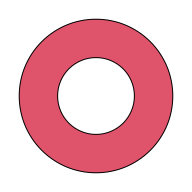
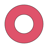
If we want to produce the same result with grid.path()
we have to construct vertices along the boundaries of the
two circles, as shown below.
t <- seq(0, 2*pi, length.out=50)
circlePts <- function(r) list(x=.5 + r*cos(t), y=.5 + r*sin(t))
c1 <- circlePts(.2)
c2 <- circlePts(.4)
grid.path(c(c1$x, c2$x), c(c1$y, c2$y), id=rep(1:2, each=50),
          rule="evenodd", gp=gpar(fill=2))
Another approach to constructing paths from shapes is provided by the 'gridGeometry' package (Murrell, 2019). For example, the concentric circle problem can be solved using this package with the following code.
library(gridGeometry)
grid.polyclip(circleGrob(r=.4,), circleGrob(r=.2), "minus",
              gp=gpar(fill=2))
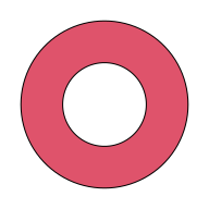
One advantage of the 'gridGeometry' approach is that it should work for all R graphics devices. However, some results, for example stroking the outline of text, that are possible with the new path features cannot be (easily) achieved with 'gridGeometry'.
In graphics systems like PostScript, the Adobe Portable Document Format, the Cairo Graphics library, and SVG, a path can be constructed from a collection of path operations: move to a point, add a straight line from the current point to a new point, or add an arc, or a (cubic) Bezier curve, or "close" a path with a straight line back to the starting point. A path may also consist of multiple subpaths, with a "move" beginning a new subpath.
The interface described in this report demonstrates that we can construct a path by adding complete subpaths based on shapes like circles, rectangles, and polygons.
The 'grid' interface also provides grid.move.to() and
grid.line.to() to construct a path from straight line
segments and there is also a function to draw stand-alone Bezier curves,
grid.bezier().
However, a small piece of future work would involve
adding a "curve to" interface that
provides a way to add an arc or a Bezier curve
to the current point in a path.
The examples and discussion in this report relate to the development version of R (specifically revision 81125), which will probably become R version 4.2.0.
This report was generated within a Docker container (see Resources section below).
Murrell, P. (2021). "Stroking and Filling Paths in R Graphics" Technical Report 2021-03, Department of Statistics, The University of Auckland. Version 1. [ bib | DOI | http ]

This document
by Paul
Murrell is licensed under a Creative
Commons Attribution 4.0 International License.