Improved Clipping in the R Graphics Engine

Version 1: original publication (Sunday 07 June 2020)
Version 2: change to dev->deviceClip (from dev->canClip=NA_LOGICAL)

This report describes improvements to clipping in the R graphics engine. These changes will be of particular interest to maintainers of R graphics device packages and to maintainers of R packages that perform visual difference testing.

1. Introduction

The R graphics engine maintains a (rectangular) clipping region; any drawing that occurs outside of the clipping region is not rendered.

The clipping region is not normally explicitly controlled by the user, but is set implicitly by plotting functions. For example, the following code draws a scatterplot with a text label below each point. When drawing the points and the text labels, the clipping region is set to be just the data region of the plot, so some of the labels are clipped. Conversely, when drawing the axes, the clipping region is reset to be the whole page, so that labels and tick marks can be drawn outside the data region of the plot.

  plot(mpg ~ disp, mtcars, pch=21, bg="grey")
  text(mpg ~ disp, mtcars, label=rownames(mtcars), pos=1, col=hcl(0, 80, 60))

The user is also able to explicitly control the clipping region. In the following code, before drawing the text labels, the par function is used to set the xpd graphics parameter so that the clipping region is the whole page. This allows the labels to be drawn outside the plot region.

  plot(mpg ~ disp, mtcars, pch=21, bg="grey")
  par(xpd=NA)
  text(mpg ~ disp, mtcars, label=rownames(mtcars), pos=1, col=hcl(0, 80, 60))

There is also a clip function in base graphics, to set the clip region to a subset of the data region of a plot, and, in the 'grid' graphics system, drawing can be clipped to any (unrotated) viewport and there is a grid.clip function for setting the clipping region within a viewport.

The following code shows an example of deliberately controlling the clipping region with the clip function. We create a blank plot and generate x and y values representing a Gaussian curve. We set the clip region to limit output to the x-range -1.96 to 1.96 and fill a polygon under the curve, which gets clipped to that x-range. Then we set the clip region back to the full data region of the plot and draw a line all the way along the curve. A small detail is that the thick black line is partially clipped as it asymptotes to the line of the x-axis. It is this sort of detailed control that clipping is useful for, but this is also where problems with the R graphics engine clipping can become apparent.

  par(mar=c(4, 2, 2, 2), yaxs="i")
  plot.new()
  plot.window(c(-4, 4), c(0, .4))
  x <- seq(-4, 4, .01)
  y <- dnorm(x)
  clip(-1.96, 1.96, 0, .4)
  polygon(x, y, col="grey", border=NA)
  axis(1, col="grey", col.axis="grey")
  clip(-4, 4, 0, .4)
  lines(x, y, lwd=3)

Most graphics devices are capable of clipping output, but the R graphics engine always performs some clipping itself before it sends output to the graphics device. One reason for this is that some graphics devices, e.g., the xfig device, are not capable of clipping output, so R must attempt to send output that is already clipped.

Another, historical, reason for the R graphics engine performing its own clipping is that the viewers for some output formats, e.g., the ghostview viewer for PostScript files, were at one time unable to cope with very large values.

2. Problems

Unfortunately, there are several problems with the clipping that the R graphics engine performs, as we will demonstrate in this section.

We will just use clipping of polygons to demonstrate the problems, both because that is where the problems are at their worst and because it is easy to demonstrate the problems with polygons. It is important to point out that the problems affect more than just polygons and also that polygons are themselves useful in R plots. The filled area under the Gaussian curve from the previous section is one example; another example is the geom_ribbon function in 'ggplot2' (Wickham, 2016) that is used to draw confidence bands.

This section will also make use of the 'grid' graphics system, again because it is easier to produce simple demonstrations, but the R graphics engine clipping affects both 'graphics' and 'grid' packages.

Clipping to the edge of the device

The first problem is that clipping to the edges of the graphics device (to avoid very large values) is too conservative.

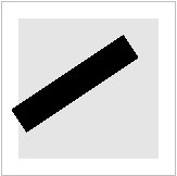
The following code provides a simple demonstration. We use the 'grid' package to draw a simple line segment that starts outside the left edge of the graphics device and ends towards the top-right of the device.

The R graphics engine clips the line to the edge of the device and, because we drew the line very thick and enforced a "butt" ending, we can clearly see the end of the clipped line.

  library(grid)
  grid.segments(-.1, .2, .8, .8,
                gp=gpar(lwd=30, lineend="butt"))

Clipping filled polygons

Another problem with clipping in the R graphics engine is that filled polygons that are clipped to the edge of the graphics device produce a border along the edge of the graphics device.

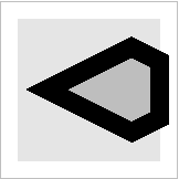
The following code draws a polygon that extends past the right edge of the device. The graphics engine clips the polygon to the edge of the device, but because we drew the polygon with a thick border, we see the clipped border running down the edge of the device.

  library(grid)
  grid.polygon(c(.2, .8, 1.4, .8),
               c(.5, .2, .5, .8),
               gp=gpar(lwd=20, fill="grey"))

Clipping empty polygons

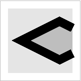
A more subtle problem occurs when the graphics engine clips an empty polygon to the edge of the device. In this case, in order to avoid drawing an edge down the side of the device, the polygon is converted to a polyline, but that produces problems of its own.

In the following code, we draw a polygon with no fill and a "mitre" line join style, which means that the corners of the polygon should be pointy, rather than rounded. When the polygon is clipped by the graphics engine, it gets converted to a polyline and, because that polyline starts and ends within the device (the left corner of the polygon), and because we drew a thick, translucent border, we can see the ends of the polyline. The default end style for the start and end of the polyline is "round", so the left corner of the polygon appears round, and the border is translucent so we can see where the start and end of the polyline overlap.

  library(grid)
  grid.polygon(c(.2, .8, 1.4, .8),
               c(.5, .2, .5, .8),
               gp=gpar(lwd=20, linejoin="mitre",
                       col=rgb(0,0,0,.5), fill=NA))

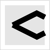
The following code and output may make the effect more obvious; here we change the line end style to "butt". The original polygon has been converted to a polyline that starts and ends at the left corner of the polygon (with two square ends). Furthermore, the polyline is clipped to the edge of the device, so we also see the square ends of the clipped polyline at the right edge of the device.

  library(grid)
  grid.polygon(c(.2, .8, 1.4, .8),
               c(.5, .2, .5, .8),
               gp=gpar(lwd=20, linejoin="mitre", lineend="butt",
                       col=rgb(0,0,0,.5), fill=NA))

3. Solutions

Several changes have been made to the R graphics engine to improve the clipping results.

dev->deviceClip

The most significant change to the graphics engine is that graphics devices can now signal that they would like to handle all clipping operations for themselves. Each graphics device has a new deviceClip flag, which is a TRUE or FALSE value to indicate whether the device wishes to perform all clipping by itself.

One advantage of this change is that there is no chance for the R graphics engine to make any mistakes or to introduce any artifacts when it clips output. There may also be performance gains because the R graphics engine will no longer be performing any clipping calculations.

There is also a new deviceVersion field so that the graphics device can indicate which graphics engine version the device supports. The graphics engine will only check the deviceClip flag if the graphics device supports a graphics engine version of 14 or above.

dev->canClip = TRUE

For existing devices that can clip (canClip=TRUE), the graphics engine still clips output to avoid very large values, but it now does this to a region well beyond the edges of the graphics device.

This change solves the first two problems from the previous section: thick lines may be clipped, but we will not see the end of the clipped line at the edge of the device; and polygons with thick borders may be clipped, but we will not see the clipped polygon border along the edge of the device.

dev->canClip = FALSE

For devices that cannot clip for themselves (canClip=FALSE), the R graphics engine will also perform clipping within the device area. In this case, we have all of the same problems as for clipping to the edges of the device. The following examples provide demonstrations using the xfig device. In the output of these examples, the device region is represented by a grey border and the region that we are clipping to is represented by a smaller grey-filled rectangle.

We will see the ends of lines that are clipped to a region within the device area. This problem remains.

  library(grid)
  grid.segments(-.1, .2, .8, .8,
                gp=gpar(lwd=30, lineend="butt"))

We also see the border of polygons that are clipped to a region within the device.

  library(grid)
  grid.polygon(c(.2, .8, 1.4, .8),
               c(.5, .2, .5, .8),
               gp=gpar(lwd=20, fill="grey"))

That problem has been improved by drawing the fill and border of the polygon separately and converting the polygon border to a polyline border.

We also see overlapping line ends when an empty polygon is converted to a polyline.

  library(grid)
  grid.polygon(c(.2, .8, 1.4, .8),
               c(.5, .2, .5, .8),
               gp=gpar(lwd=20, linejoin="mitre", fill=NA))

This problem has been improved by reordering the vertices of the converted polyline so that it begins outside the clipping region (so that all vertices within the clipping region are joins rather than line ends).

This also solves the problem for devices that can clip for themselves for the very rare cases where a polygon extends well beyond the edges of the device so that the R graphics engine clips the output anyway.

4. Impacts on R packages

The addition of dev->deviceClip may be of interest to developers of R graphics device packages, e.g., the 'Cairo' package (Urbanek and Horner, 2020), in case there are performance gains to be had.

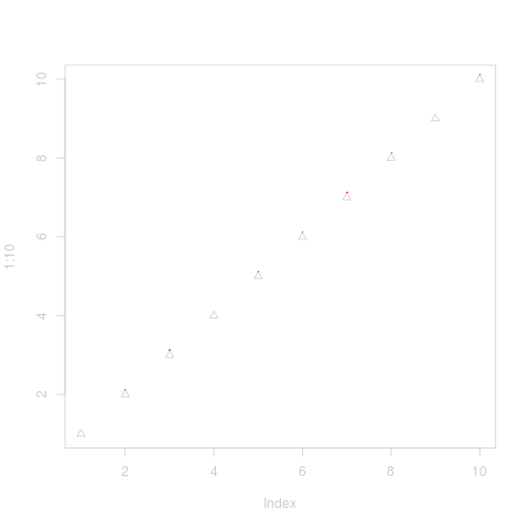
Packages that conduct visual difference testing, e.g., with 'vdiffr' (Henry et al., 2019) or 'gdiff' (Murrell, 2020a, Murrell, 2020b), may notice minor changes and may need to update their "model" output. For example, the code below shows the effect of these clipping changes on a simple scatterplot (comparing R 3.6.3 with the development version of R).

library(gdiff)
f <- function() plot(1:10, pch=2)
gdiff(f,
      device=pngDevice(type="cairo"),
      session=list(control=localSession(Rpath="Rscript"),
                   test=localSession(Rpath="/R/bin/Rscript")))

  
  Files that differ [1/1]
  ----------------------------------------------------------------------------------------------------
  Control/f-001.png differs from Test/f-001.png (Compare/f-001.png.png [9])

The differences are small (see the red dots in the image of the differences below), but will show up in visual difference testing like this.

5. Summary

The clipping that is performed by the R graphics engine has been improved so that there are fewer artifacts produced by this clipping. It is now also possible for a graphics device to indicate, via dev->deviceClip = TRUE, that it does not want the graphics engine to perform any clipping at all.

6. Acknowledgements

This work was partially supported by a donation from R Studio to The University of Auckland Foundation. Thanks to Thomas Lin Pedersen for the initial reports about problems with the R graphics engine clipping.

7. Technical requirements

The examples and discussion in this report relate to the development version of R (specifically revision 79409), which will become R version 4.1.0. The examples of "old" clipping behaviour were produced using R version 3.6.3.

This report was generated within a Docker container (see Resources section below).

8. Resources

How to cite this report

Murrell, P. (2020). "Improved Clipping in the R Graphics Engine" Technical Report 2020-03, Department of Statistics, The University of Auckland. Version 2. [ bib | DOI | http ]