This document describes an extension of the support for pattern fills in R graphics (linear gradients, radial gradients, and tiling patterns) to allow multiple pattern fills to be specified at once when drawing.

Gradient fills and pattern fills are currently only available on the pdf() and Cairo-based graphics devices, of the core graphics devices provided by the 'graphics' package, plus the graphics devices provided by the 'ragg' package (Pedersen and Shemanarev, 2021) and the 'svglite' package (Wickham et al., 2022).

1. Introduction

Changes to the graphics engine in R 4.1.0 added support for pattern fills, clipping paths, and masks (Murrell, 2020). The patterns that are currently supported are linear gradients, radial gradients, and tiling patterns. The following example demonstrates the use of a linear gradient to fill a rectangle. In this case, we have a gradient from black to white and back again several times.

colours <- c("black", "white", "black", "white", "black")
gradient <- linearGradient(colours)
grid.rect(width=.8, height=.8,
          gp=gpar(fill=gradient))

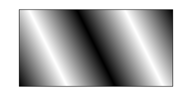
The expected behaviour is reasonably clear when drawing a single shape like the single rectangle above; the linear gradient is relative to the dimensions of the rectangle (by default, from bottom-left to top-right). However, it is possible for a single call to grid.rect() to draw more than one rectangle. What should happen then?

What currently happens is shown below: the linear gradient is relative to a bounding box around all of the rectangles that are drawn (as indicated by the green rectangle in the output below).

grid.rect(x=c(.1, .4, .7), y=c(.1, .3, .5), width=.2, height=.4,
          just=c("left", "bottom"),
          gp=gpar(fill=gradient))

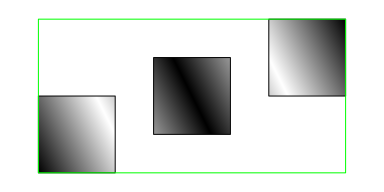
This might be what we want to have happen, but there are other possible outcomes. For example, we might want to fill each individual rectangle separately with its own linear gradient.

This document describes an extension of the 'grid' support for pattern fills that allows for more control over the behaviour of pattern fills when we are drawing more than one shape.

2. Vectorised pattern fills

The functions linearGradient(), radialGradient(), and pattern() all have a new argument called group. By default, this argument is TRUE, which means that the pattern fill is relative to the "group" of shapes that are being drawn, as shown above.

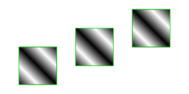
However, if we specify group=FALSE, then the pattern fill is drawn relative to each individual shape that is being drawn. For example, the code below draws the same three rectangles as the previous example, and uses the same linear gradient as before except that group=FALSE. Each rectangle is now filled with the gradient relative to the individual rectangle (as indicated by the green rectangles).

gradient2 <- linearGradient(colours, group=FALSE)
grid.rect(x=c(.1, .4, .7), y=c(.1, .3, .5), width=.2, height=.4,
          just=c("left", "bottom"),
          gp=gpar(fill=gradient2))

It is also now possible to specify a list of pattern fills rather than just a single pattern fill. For example, the following code defines a linear gradient, a radial gradient, and a polka dot tiling pattern.

pat1 <- linearGradient(colours)
pat2 <- radialGradient(colours)
pat3 <- pattern(circleGrob(r=unit(1, "mm"), gp=gpar(fill="black")),
                width=unit(3, "mm"), height=unit(3, "mm"),
                extend="repeat")

The following code draws three rectangles and specifies a list of three pattern fills. The result is that each rectangle uses a different pattern fill.

grid.rect(x=c(.1, .4, .7), y=c(.1, .3, .5), width=.2, height=.4,
          just=c("left", "bottom"),
          gp=gpar(fill=list(pat1, pat2, pat3)))

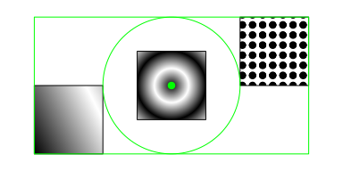
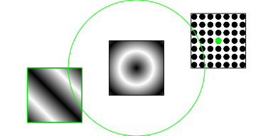
However, the three pattern fills above are still each relative to the bounding box around all of the rectangles. This is indicated by the green rectangle (for the linear gradient), the green circle (for the radial gradient), and the green dot (which is the basis of the tiling pattern).

We can change this behaviour using the new group argument. For example, the following code defines three new patterns, very similar to the previous three patterns, but with group=FALSE.

pat4 <- linearGradient(colours, group=FALSE)
pat5 <- radialGradient(colours, group=FALSE)
pat6 <- pattern(circleGrob(r=unit(1, "mm"), gp=gpar(fill="black")),
                width=unit(3, "mm"), height=unit(3, "mm"),
                extend="repeat", group=FALSE)

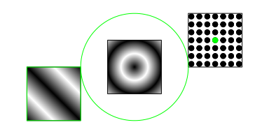
The following code draws the same three rectangles as before, specifies the list of three new patterns as the fill, and the result is that each pattern is filled with its own pattern and each pattern is relative to its individual rectangle (again indicated by a green rectangle, circle, and dot).

grid.rect(x=c(.1, .4, .7), y=c(.1, .3, .5), width=.2, height=.4,
          just=c("left", "bottom"),
          gp=gpar(fill=list(pat4, pat5, pat6)))

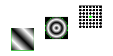
It is also possible to specify a list of patterns, some of which are "grouped" and some of which are not. The following code demonstrates this by drawing three rectangles with a linear gradient (not grouped), a radial gradient (grouped), and a tiling pattern (not grouped). The linear gradient is relative to the first rectangle (bottom-left), the radial gradient is relative to the bounding box of all three rectangles, and the tiling pattern is relative to the third rectangle (top-right).

grid.rect(x=c(.1, .4, .7), y=c(.1, .3, .5), width=.2, height=.4,
          just=c("left", "bottom"),
          gp=gpar(fill=list(pat4, pat2, pat6)))

In summary, it is now possible to specify a "vector" of pattern fills, just like being able to specify a vector of fill colours, or line widths, or font sizes. Only as many patterns are used as there are shapes to fill (the remainder are ignored) and patterns are recycled if necessary. Furthermore, when we draw a grob that produces more than one shape, the new group argument allows the pattern fills to be resolved relative to individual shapes rather than an overall bounding box.

3. Data symbols with pattern fills

Another improvement to the 'grid' support of pattern fills is the ability to fill data symbols, as drawn by grid.points() (this was not possible in R 4.1.0). If we combine this with the ability to fill individual shapes, we can fill individual data symbols with pattern fills. For example, the following code defines a radial gradient (with group=FALSE) and then fills the data symbols on a 'ggplot2' plot (Wickham, 2016) with that gradient. The 'ggplot2' package does not yet have an interface for pattern fills, but the 'gggrid' package (Murrell, 2022) allows us to combine raw 'grid' output with the 'ggplot2' plot.

gradient <- radialGradient(c("white", "black"), cx1=.7, cy1=.7, group=FALSE)
ggplot(mtcars, aes(x=disp, y=mpg)) +
    grid_panel(function(data, coords) {
                   pointsGrob(coords$x, coords$y, pch=21,
                              gp=gpar(fill=gradient, col=NA))
               })

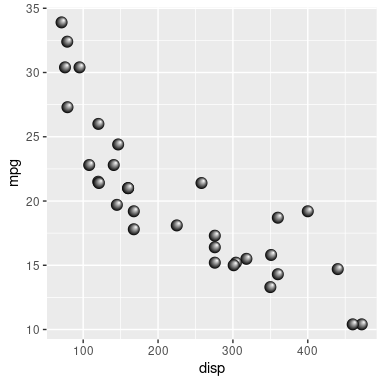
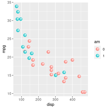
In the example above, we defined a single radial gradient and recycled that gradient across multiple data symbols. The next example generates a separate gradient for each data symbol based on a categorical variable (and a colour that is selected by 'ggplot2'). This shows that it can be easy to generate a list of pattern fills with functions like lapply(). This example also uses 'gggrid' to draw points with gradients in the legend.

gradientPoints <- function(data, coords) {
    gradients <- lapply(data$colour,
                        function(x) {
                            radialGradient(c("white", x),
                                           cx1=.7, cy1=.7,
                                           group=FALSE)
                            })
    pointsGrob(coords$x, coords$y, pch=21,
               gp=gpar(fill=gradients, col=NA))
}
gradientKey <-  function(data, ...) {
    gradient <- radialGradient(c("white", data$colour), cx1=.7, cy1=.7,
                               group=FALSE)
    pointsGrob(.5, .5, pch=21,
               gp=gpar(fill=gradient, col=NA))
}
mtcars$am <- as.factor(mtcars$am)
ggplot(mtcars) +
    grid_panel(gradientPoints,
               mapping=aes(x=disp, y=mpg, colour=am),
               key_glyph=gradientKey, show.legend=TRUE)

4. Pattern fills on viewports

As well as being able to specify a pattern fill on a grob, it is also possible to specify a pattern fill on a 'grid' viewport.

The graphical parameter settings of a viewport provide a "graphical context" for any drawing within the viewport. If a grob is drawn without its own explicit graphical parameter settings, it will "inherit" the settings from its parent viewport. For example, the code below will produce a rectangle filled with red because, although the grid.rect() call says nothing about the fill colour, the rectangle is drawn within a viewport that sets fill=2 (and the second colour in the default palette is red).

pushViewport(viewport(gp=gpar(fill=2)))
grid.rect()

When the fill parameter is a pattern fill things are a little more complicated. By default, if the pattern fill has group=TRUE, the pattern is relative to the extent of the viewport, so any drawing within the viewport inherits a pattern relative to the viewport (unless a grob specifies its own fill setting).

For example, the following code draws the three rectangles as in previous examples, using three group=TRUE patterns (pat1, pat2, pat3), but with the list of pattern fills specified on the viewport within which the rectangles are drawn (rather than being specified directly in the grid.rect() call).

pushViewport(viewport(gp=gpar(fill=list(pat1, pat2, pat3))))
grid.rect(x=c(.1, .4, .7), y=c(.1, .3, .5), width=.2, height=.4,
          just=c("left", "bottom"))

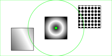
The three rectangles each use a different pattern fill because the graphical context set up by the viewport has specified a list of three pattern fills, but all three pattern fills are relative to the viewport (as indicated by the green rectangle, circle, and dot). This result is slightly different from when we specified the three patterns directly in the grid.rect() call because the viewport (which takes up the whole image) is a little larger than the bounding box around the three rectangles.

We can also specify patterns on a viewport with group=FALSE. In this case, any drawing within the viewport inherits a pattern that is drawn relative to individual shapes. A mixture of grouped and ungrouped patterns is also possible.

For example, the following code pushes a viewport with three pattern fills, the first an ungrouped linear gradient, the second a grouped radial gradient, and the third an ungrouped tiling pattern. The three rectangles that are drawn within the viewport inherit, respectively, a linear gradient relative to the first rectangle, a radial gradient relative to the viewport, and a tiling pattern relative to the last rectangle.

pushViewport(viewport(gp=gpar(fill=list(pat4, pat2, pat6))))
grid.rect(x=c(.1, .4, .7), y=c(.1, .3, .5), width=.2, height=.4,
          just=c("left", "bottom"))

5. Pattern fills on gTrees

A gTree is a collection of grobs - when we draw a gTree, we draw all of its children - and a gTree can itself have graphical parameter settings. Like a viewport, the gTree provides a graphical context for its children so that its children inherit settings if they do not specify their own. For example, the following code draws a rectangle and a circle, both filled red, because although neither rectangle nor circle say anything about fill colour, they are children of a gTree that specifies fill=2 (and the second colour in the default palette is red).

grid.draw(gTree(children=gList(rectGrob(x=.25, width=.5),
                               circleGrob(x=.75, r=.5)),
                gp=gpar(fill=2),
                vp=viewport(width=.8, height=.8)))

If we specify a pattern fill on the gTree, the children inherit the pattern fill. For example, the following code draws a gTree with a linear gradient as the fill and a rectangle and a circle as its children. The result shows that, similar to viewports, if a pattern fill is specified on a gTree with group=TRUE, the children of the gTree inherit a pattern fill that is relative to the gTree. And "relative to the gTree" means relative to a bounding box around all of the children of the gTree.

grid.draw(gTree(children=gList(rectGrob(x=.25, width=.5),
                               circleGrob(x=.75, r=.5)),
                gp=gpar(fill=linearGradient()),
                vp=viewport(width=.8, height=.8)))

On the other hand, if a pattern fill is specified on a gTree with group=FALSE, the children of the gTree inherit a pattern fill that is relative to individual shapes drawn by the children (just like what happens for a viewport).

For example, the following code defines a gTree with three pattern fills, the first an ungrouped linear gradient, the second a grouped radial gradient, and the third an ungrouped tiling pattern. The gTree has a single grob as its child and that grob inherits the pattern fills from the gTree (because the grob does not specify its own fill). The grob draws three rectangles and they are filled with, respectively, a linear gradient relative to the first rectangle, a radial gradient relative to the gTree (a bounding box around all three rectangles), and a tiling pattern relative to the last rectangle.

gt <- gTree(children=gList(rectGrob(x=c(.1, .4, .7),
                                    y=c(.1, .3, .5),
                                    width=.2, height=.4,
                                    just=c("left", "bottom"))),
            gp=gpar(fill=list(pat4, pat2, pat6)))
grid.draw(gt)

6. Groups and paths with pattern fills

R version 4.2.0 also introduced two new graphics features: groups (Murrell, 2021a) and stroked/filled paths (Murrell, 2021b). These present interesting complications for pattern fills.

Resolving patterns on groups

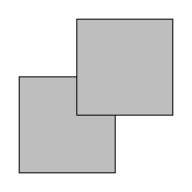
A group consists of a "source" grob combined with a "destination" grob, using a compositing operator. For example, the following code draws a group, with a grey fill, where the group consists of one rectangle combined with another rectangle using the default "over" operator (one rectangle is drawn on top of the other).

r1 <- rectGrob(.1, .1, .5, .5, just=c("left", "bottom"))
r2 <- rectGrob(.4, .4, .5, .5, just=c("left", "bottom"))
grid.group(r2, "over", r1,
           gp=gpar(fill="grey"))

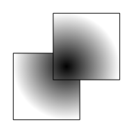
If we use a radial gradient fill on the group instead, the gradient is resolved relative to a bounding box around both the source and the destination. In the example below, the two rectangles are both being filled separately, just with the same gradient fill.

grid.group(r2, "over", r1,
           gp=gpar(fill=radialGradient()))

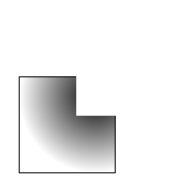
Where things get interesting is if we use a different compositing operator. In the code below, we use a "clear" operator, so the source erases the destination where the two overlap (and the source is not drawn). However, the radial gradient is still resolved relative to both source and destination, so the destination is filled with a radial gradient relative to a bounding box around both itself and the (invisible) source.

grid.group(r2, "clear", r1,
           gp=gpar(fill=radialGradient()))

Another interesting scenario occurs if we separate group definition from group use. If the group use occurs within a different viewport than the group definition, a transformation is applied to the group. If the resolution of a pattern requires determining the bounding box for the group use, the bounding box is around the transformed group.

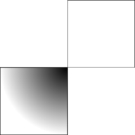
The following code demonstrates this sort of scenario. We have a grob, r3, that describes a rectangle in the bottom left quadrant of the image. We define a group called "r" based on that rectangle. This definition occurs in the default viewport that is centred on (.5, .5). We then have another grob user3 that uses the group "r" in a viewport that is centred on (1, 1). That use will translate the rectangle up to the top-right quadrant of the image. Now we define a gTree with two children: the grob r3, a rectangle in the bottom-left quadrant; and the grob user3, a rectangle in the top-right quadrant. The gTree has a radial gradient fill, which gets resolved relative to the bounding box around the gTree, which is the entire image. The result is that the rectangle at bottom-left is filled with a radial gradient that was resolved relative to the entire image. The rectangle at top-right has no fill because it is just a use of the group "r", which was defined with no fill.

r3 <- rectGrob(0, 0, .5, .5, just=c("left", "bottom"))
grid.define(r3, name="r")
user3 <- useGrob("r", vp=viewport(1, 1))
gt <- gTree(children=gList(r3, user3),
            gp=gpar(fill=radialGradient()))
grid.draw(gt)

The situation is simpler if we just specify a pattern fill on a grob within the group. In that case, the pattern is recorded normally as part of the group definition and the pattern is transformed (on the device) when the group is used.

In order for the calculation of the bounding box of a group use to work, the bounding box of the group has to be recorded when the group is defined. In cases where it is known that the group will not be reused, this calculation can be turned off using the coords argument.

Resolving patterns on stroked and filled paths

When a fill pattern is specified for a stroked or filled path, the bounding box for resolving the pattern is based on all of the grobs that define the path. This is because a stroked or filled path is conceptually just a single shape. In the example below, we fill a path that is constructed from two nested circles, using an "evenodd" rule so that the inner circle generates a hole in the outer circle. We then fill the resulting "donut" with a radial gradient, which is resolved relative to a bounding box around both circles.

grid.fill(circleGrob(r=c(.2, .4)), rule="evenodd",
          gp=gpar(fill=radialGradient()))

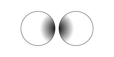
A further corollary is that group=FALSE will have no effect on the resolution of a pattern fill for a stroked or filled path. For example the code below constructs a path from two distinct circles and then fills the path with a radial gradient with group=FALSE. The path is a single shape so the radial gradient is resolved relative to a bounding box around both of the circles.

grid.fillStroke(circleGrob(x=1:2/3, r=.3),
                gp=gpar(fill=radialGradient(group=FALSE)))

7. Summary

From R version 4.2.0, we can resolve pattern fills relative to individual shapes within a grob and we can specify different pattern fills for different shapes within a grob. This means that pattern fills can now be used just like normal colour fills. This includes using pattern fills on individual data symbols.

8. Technical requirements

The examples and discussion in this report relate mostly to R version 4.2.0. Some of the examples in Groups and paths with pattern fills rely on bug fixes that require R version 4.2.1.

The 'ggplot2' example that draws points with gradients in the legend requires 'gggrid' version 0.2-0 or higher.

This report was generated within a Docker container (see Resources section below).

9. Resources

How to cite this report

Murrell, P. (2022). "Vectorised Pattern Fills in R Graphics" Technical Report 2022-01, Department of Statistics, The University of Auckland. Version 1. [ bib | DOI | http ]

Vectorised Pattern Fills in R Graphics

Table of Contents: