
Abstract
This report describes the animaker package for generating descriptions of animation sequences. An animation sequence is composed by combining atomic animations in series to create sequence animations or in parallel to create track animations. Functions are provided for manipulating animation sequences, generating timing schemes from animation sequences, and producing diagrams to visualise animation sequences.
Several R packages exist for generating animations in R. For example, the animation package provides convenience functions for generating an animation, in a wide variety of formats, from a series of static frames, where the frames are drawn in a loop using normal R graphics functions. Several other packages provide a more declarative approach, allowing individual animation actions to be specified in terms of a start value and end value (plus a start time and end time). For example, the animatoR package provides functions for generating static frames from a declarative animation and the gridSVG package and the SVGAnnotation package both provide functions for adding declarative animation information to an R plot in an SVG format (for viewing on the web).
One of the difficulties that arises when attempting to generate an animation sequence with these packages is the coordination of multiple animation actions. For example, something as simple as ensuring that action A follows action B can become complicated to specify and difficult to maintain if those two actions are part of a larger collection of animation actions that also need to be run either in sequence or in parallel.
This report describes an R package called animaker that can be used to generate a description of an animation sequence. The description is completely abstract and only focuses on a specification of when animation actions should occur. Animation actions are only represented by a label and no actions are actually carried out, though there are functions to generate a timing information for the animation. There are also functions for drawing diagrams (including animated diagrams) to visualise the animation sequence.
The fundamental component of an animation sequence is an
atomic animation, which
simply consists of a
start
value and a
durn
(duration). It is also possible to specify a
label,
but this will be automatically generated by default.
An atomic animation is generated using the
atomic()
function; both the
start
and
durn
default to zero.
atomic()
Alpha:0:0
The following code shows a more realistic example, where an atomic animation
is generated with a duration of 2 seconds. There is a
plot()
method for atomic animations which draws a diagram of
the animation sequence represented by the atomic animation
(see Figure 1, “An atomic animation”).
atmc <- atomic(durn=2)
atmc
Bravo:0:2
The
start
argument can be used to delay the start of the animation,
as shown in the code below and in Figure 2, “A delayed atomic animation”.
delay <- atomic(start=1, durn=2)
delay
Charlie:1:2
Figure 2. A diagram of an atomic animation with a delay of 1 second (and a duration of 2 seconds). (animated version)
NOTE that this system only uses the start and duration times to determine when an animation action will be started. There is no requirement that the animation action actually plays for exactly the prescribed duration. It is expected that the duration will be passed to the animation action and that some actions will take note of the duration and respond accordingly, but it is also acknowledged that the animation action may completely ignore the duration information.
A container animation is a collection of animations. In the simplest case, a container is a collection of atomic animations, but it is also possible to have a collection of container animations (or a mixture of both).
There are two sorts of containers, sequence animations and track animations. A sequence animation plays a collection of animations one after the other. A track animation plays a collection of animations simultaneously.
To demonstrate these ideas, we first create three atomic animations: one lasting 1 second, one lasting 2 seconds, and one lasting 3 seconds.
a <- atomic(durn=1)
b <- atomic(durn=2)
c <- atomic(durn=3)
The
vec()
function can be used to create a sequence animation by running these
animations sequentially (see Figure 3, “A sequence animation”)
v <- vec(a, b, c)
The
trac()
function can be used to create a track animation by running these
animations in parallel (see Figure 4, “A track animation”)
t <- trac(a, b, c)
The contents of a container can be another container. For example, the following code produces an animation sequence consisting of a track animation followed by a sequence animation (see Figure 5, “A container animation”)
container <- vec(t, v)
Figure 5. A sequence animation consisting of a track animation followed by a sequence animation. (animated version)
A container animation may have its own
start,
which delays the entire collection of animations
(see Figure 6, “A delayed sequence animation”).
vDelay <- vec(a, b, c, start=1)
Figure 6. A sequence animation (consisting of three atomic animations) with a delayed start. (animated version)
By default, the
durn
of a container animation is calculated from the animations within the
container, but this may be overridden
(see Figure 7, “A sequence with explicit duration”).
vDurn <- vec(a, b, c, start=1, durn=10)
Figure 7. A sequence animation (consisting of three atomic animations) with a delayed start and an explicit duration. (animated version)
For the contents
of a sequence animation, the start value
represents a delay that is relative to the
end of the previous animation in the sequence.
For example, the following code generates an atomic animation
that starts after a delay of 0.5 seconds and lasts for 2 seconds.
If this animation is used as part of an animation sequence,
the delay on the atomic animation creates a pause within the sequence
(see Figure 8, “Delayed content within a sequence”).
d <- atomic(start=.5, durn=2)
vContentDelay <- vec(a, b, c, d)
Figure 8. A sequence animation (consisting of four atomic animations) where the fourth atomic animation has a delay. (animated version)
For the contents of track animations, a delay is just relative to the start of the track animation. For example, the following code generates a track animation from two atomic animations where the second atomic animation has a delay of 0.5 seconds so it starts after the first atomic animation (see Figure 9, “Delayed content within a sequence”).
tContentDelay <- trac(a, d)
Figure 9. A sequence animation (consisting of four atomic animations) where the fourth atomic animation has a delay. (animated version)
It is also possible for the container to override the
start and duration values for its contents.
This is achieved by specifying a vector of values for
either
start
or
durn.
The following code shows this feature being used
to insert a delay between animations within a sequence.
There are three atomic animations in the sequence, each of which
has a start of zero, but the sequence
animation specifies
start
values of 0, 0.5, and 0.5, which override the atomic animation start values
(see Figure 10, “Parent delayed content within a sequence”).
vParentDelay <- vec(a, b, c, start=c(0, .5, .5))
Figure 10. A sequence animation (consisting of three atomic animations) where the parent sequence has inserted a delay between the atomic animations. (animated version)
The following code combines the three atomic animations into a
track animation where the track animation specifies
start
values for the atomic animations in order
to stagger the start of the animations within the track
(see Figure 11, “Parent delayed content within a track”).
tParentDelay <- trac(a, b, c, start=c(0, .5, 1))
Figure 11. A track animation (consisting of three atomic animations) where the parent track has staggered the start of the atomic animations. (animated version)
An example of the container explicitly controlling the duration of its contents will be shown later in the section called “Examples”.
Another possibility is that an atomic animation may abdicate
responsibility for its duration to its parent container.
This is achieved by specifying
NA
for the
durn
of an atomic animation.
This only works if the container animation is not also
relying on calculating its duration from its contents.
In the case of a sequence animation, if the container has
an explicit duration
then any atomic content of the container can have
NA
duration, in which case the container duration is equally
shared out amongst such atomic content.
In the case of a track animation, if either the container
has an explicit duration or at least one animation in the contents
of the container has an explicit duration (from which the
container can calculate its duration), then
any atomic content with
NA
duration is given the container duration.
For example, the following code generates a sequence animation
from five atomic animations, where the second and fourth
atomic animations have
NA
duration. The sequence animation has an explicit duration of
10 seconds, three of the atomic animations have a combined
duration of 6 seconds, so the two atomic animations with
NA
duration get 2 seconds each (4 seconds divided by 2).
f <- atomic(durn=NA)
navec <- vec(a, f, b, f, c, durn=10)
Figure 12. A sequence animation consisting of five atomic animations,
where the second and fourth atomic animations have a
duration of
NA,
so their duration is calculated from the parent sequence.
(animated version)
In the following code, a track animation is generated
from four atomic animations, with the fourth atomic animation
having
NA
duration. The fourth atomic animation gets the same duration
as the longest of the atomica animations with a known duration.
natrac <- trac(a, b, c, f)
Figure 13. A track animation consisting of four atomic animations,
where the fourth atomic animation has a
duration of
NA,
so its duration is calculated from the longest of the atomic
animations with a known duration.
(animated version)
Several useful manipulations are possible on container animations.
For example, there is a
rep()
method to generate regular patterns of animation actions.
The following code shows a sequence animation being repeated
three times
(see Figure 14, “A repeated sequence”).
vRep <- rep(v, 3)
Figure 14. A sequence animation (consisting of three atomic animations) repeated three times. (animated version)
Notice that the result of repeating a container is just a container with the original contents repeated (not a container with the original container repeated). The result of repeating an atomic animation is special and it produces a container animation (by default a sequence, but a vec argument allows the result to be a track animation instead).
It is also possible to subset a container. Single square brackets produce a smaller version of the original container, consisting of a subset of the original contents, and double square brackets produce a single item from the original contents. The following code shows various subsets being generated from a sequence animation.
vRep
Delta:0:1|Echo:0:2|Foxtrot:0:3|Delta:0:1|Echo:0:2|Foxtrot:0:3|Delta:0:1|Echo:0:2|Foxtrot:0:3
vRep[2]
Echo:0:2
class(vRep[2])
[1] "vecAnim" "containerAnim" "anim"
vRep[[2]]
Echo:0:2
class(vRep[[2]])
[1] "atomicAnim" "anim"
vRep[3:5]
Foxtrot:0:3|Delta:0:1|Echo:0:2
vRep[c(TRUE, FALSE)]
Delta:0:1|Foxtrot:0:3|Echo:0:2|Delta:0:1|Foxtrot:0:3
vRep[rep(2:3, 2)]
Echo:0:2|Foxtrot:0:3|Echo:0:2|Foxtrot:0:3
Assignment to a subset of a container animation is also possible, using both single and double square brackets. The value being assigned must be compatible with the container so, for example, only a sequence animation can be assigned to a subset of a sequence animation, and an atomic animation may only be assigned using double square brackets.
Finally, there is a
splice()
function for inserting new content into a container animation.
Both atomic animations and container animations may be
inserted into a container.
For example, the following code appends an atomic animation onto
the end of a sequence animation of three atomic animations
to make a sequence of four atomic animations
(see Figure 15, “Appending to a sequence”)
and then splices in a track animation after position 2 in the sequence
(see Figure 16, “Splicing a sequence”).
e <- atomic(durn=1)
vAppend <- splice(v, e)
Figure 15. A sequence animation (consisting of three atomic animations) with a fourth atomic animation appended. (animated version)
vSplice <- splice(vAppend, t, after=2)
Figure 16. A sequence animation (consisting of four atomic animations) with a track animation spliced in after the second atomic animation. (animated version)
In addition to the
after
argument to
splice(),
which allows animations to be inserted in between existing
animations in a sequence or track,
there is also an
at
argument to
splice(),
which allows animations to be inserted alongside
existing animations in a sequence or track.
For example, the following code splices an atomic animation
into a sequence animation at position 2.
The result is a sequence that splits into two tracks at position 2;
one track has the original remainder of the sequence and the other
track has the spliced in atomic animation
(see Figure 17, “Splicing alongside a sequence”).
sequence <- vec(a, b, c)
newSeq <- splice(sequence, e, at=2)
Figure 17. A sequence animation (consisting of three atomic animations) with a new atomic animation spliced in alongside the second atomic animation in the original sequence. (animated version)
The ultimate purpose of constructing an animation description is
to be able to coordinate the timing of multiple animation actions.
The
timing()
function is provided to turn an animation description into
a timing scheme.
The following code shows the simplest case for an atomic animation.
This shows the basic information that is produced for each atomic
animation: the label of the animation, when it starts and its duration
(the animation diagram is also shown in Figure 18, “An atomic animation”
for comparison).
timing(a)
  label start durn vec vecNum trac tracNum
1 Delta 0     1
Figure 18. A simple atomic animation that starts at after 0 seconds and lasts for 1 second. (animated version)
The next example shows the timing information from a sequence animation (consisting of three atomic animations; see Figure 19, “A sequence animation”). The first thing to note is that there is a line of timing information for each atomic animation. Secondly, in addition to the basic start and duration information, there is information about the context in which the atomic animation occurs. In particular, the context tells us the sequence animation and the track animation in which each atomic animation occurs, plus which iteration within the sequence animation and which track within the track animation the atomic animation represents. In this case, the atomic animations are the first, second, and third iterations within a single sequence animation (and there are no tracks).
timing(v)
  label   start durn vec  vecNum trac tracNum
1 Delta   0     1    Golf 1
2 Echo    1     2    Golf 2
3 Foxtrot 3     3    Golf 3
The next example shows a more complex animation, consisting of a sequence animation made up from a sequence animation followed by a track animation (see Figure 20, “A container animation”). One complication is that there are now many atomic animations to give timing information for. There is also a lot more context information to convey for each atomic animation. For example, the third atomic animation starts after 0 seconds and lasts for 3 seconds. This atomic animation is part of the first iteration within a sequence and it is on the third track of a track animation. The fourth atomic animation starts after 3 seconds and lasts for 1 second. This atomic animation is the first iteration within a sequence, which is itself the second iteration within a parent sequence.
timing(container)
  label   start durn vec        vecNum trac  tracNum
1 Delta   0     1    India      1      Hotel 1
2 Echo    0     2    India      1      Hotel 2
3 Foxtrot 0     3    India      1      Hotel 3
4 Delta   3     1    India:Golf 2:1
5 Echo    4     2    India:Golf 2:2
6 Foxtrot 6     3    India:Golf 2:3
Figure 20. A sequence animation that consists of a track animation followed by a sequence animation. (animated version)
Although the timing information for this example is relatively complex, it is still straightforward to extract the basic information for any atomic animation. The information for the overall animation is structured as a list, with one component for each atomic animation. The information for each atomic animation is itself just a list of seven components. For example, the following code shows how we can easily extract just the start time and duration for the fourth atomic animation.
tim <- timing(container)
tim[[4]]$start
[1] 3
tim[[4]]$durn
[1] 1
It is also important to note that the context information is stored as a vector of information for each atomic animation. For example, the following code shows the sequence context for the fourth atomic animation.
tim[[4]]$vec
[1] "India" "Golf"
tim[[4]]$vecNum
[1] 2 1
It is therefore possible to use this contextual information programmatically to determine useful information about when within a larger animation a particular atomic animation occurs.
Another way to access timing information is to ask which atomic animations are active at a particular time point. This sort of information is more useful for generating an animation as a series of static frames because it provides information about what to draw within each frame.
The frameTiming() function
returns timing information for atomic animations that are active
at a specific time point. For example, the following code tells
us that, after 1.5 seconds of the
container
sequence animation, atomic animations
b and
c are active
(within track 2 and track 3 of the first step in the parent sequence,
respectively;
see Figure 20, “A container animation”)
and after 5 seconds only
b is active
(this time as step 2 of the sequence within step 2 of the parent sequence
see Figure 20, “A container animation”).
frameTiming(container, 1.5)
  label   start durn vec   vecNum trac  tracNum
1 Echo    0     2    India 1      Hotel 2
2 Foxtrot 0     3    India 1      Hotel 3
frameTiming(container, 5)
  label start durn vec        vecNum trac tracNum
1 Echo  4     2    India:Golf 2:2
A frameApply() is also provided
to call a user-specified function on the timing information
for an animation at a set of time points (frames) spanning the
entire animation. The default is just to print the
timing information for each frame, but this can be used to draw
the content for each frame (an example is given in
the section called “Examples”).
The following code shows the default output from
frameApply()
for the simple sequence animation v
with one frame per second.
capture.output(frameApply(v, pause=FALSE))
 [1] "  label start durn vec  vecNum trac tracNum"
 [2] "1 Delta 0     1    Golf 1                  "
 [3] "  label start durn vec  vecNum trac tracNum"
 [4] "1 Echo  1     2    Golf 2                  "
 [5] "  label start durn vec  vecNum trac tracNum"
 [6] "1 Echo  1     2    Golf 2                  "
 [7] "  label   start durn vec  vecNum trac tracNum"
 [8] "1 Foxtrot 3     3    Golf 3                  "
 [9] "  label   start durn vec  vecNum trac tracNum"
[10] "1 Foxtrot 3     3    Golf 3                  "
[11] "  label   start durn vec  vecNum trac tracNum"
[12] "1 Foxtrot 3     3    Golf 3                  "
A
plot()
method is defined for animations and this was used to produce
all of the figures in this report.
There is also a
dynPlot()
function, which draws a dynamic (SVG) version of the diagram
in which each rectangle is animated appropriately
(see the links to "animated version" in each figure caption).
This section provides some demonstrations of how these functions could be used to construct animations.
The first example shows a sequence being constructed from many repetitions of an atomic animation. The idea here is that there is an atomic animation that is demonstrated a few times slowly, then again a bit faster, and a third time very fast. The atomic animation is identical each time and the container varies the duration (see Figure 21, “A long sequence”).
r <- rep(a, 15)
durn(r) <- rep(c(10, 5, 1), each=5)
Figure 21. A sequence animation (consisting of four atomic animations) with a track animation spliced in after the second atomic animation. (animated version)
A gridSVG example
The next example produces an actual animation, based on the Pong computer game. The following code uses the grid package to draw a simple solo Pong playing field, with three walls, a ball, and a paddle (see Figure 22, “A Pong playing field”).
pushViewport(viewport(width=.8, height=.8))
# Walls
grid.segments(c(1, 0, 0), c(0, 0, 1),
              c(0, 0, 1), c(0, 1, 1))
# Paddle
grid.rect(unit(1, "npc") + unit(2, "mm"),
          width=unit(4, "mm"),
          height=unit(2, "cm"),
          just="left",
          gp=gpar(fill="black"),
          name="paddle")
# Ball
grid.circle(1, .5, r=unit(2, "mm"),
            gp=gpar(fill="black"),
            name="ball")
The idea of the animation is that the Pong ball will cycle around the field in a simple pattern while the Pong paddle performs various "tricks". The overall animation will be constructed from a Pong ball animation (repeated six times) and three different Pong paddle animations, with the ball and paddle in separate tracks, but coordinated at every second repetition of the ball animation (see Figure 23, “A Pong animation sequence”).
ballMove <- atomic(label="ball", durn=3)
paddleMove <- atomic(label="paddle", durn=3)
sequence <- rep(vec(ballMove, trac(paddleMove, ballMove)), 3)
sequence
ball:0:3|paddle:0:3|ball:0:3|paddle:0:3|ball:0:3|paddle:0:3
        |ball:0:3  |        |ball:0:3  |        |ball:0:3
Figure 23. A sequence animation consisting of an atomic animation followed by a track animation, repeated four times. (animated version)
This description of the steps in the animation allows us to generate a timing scheme for the actual animation actions, as shown below.
tim <- timing(sequence)
tim
  label  start durn vec   vecNum trac  tracNum
1 ball    0    3    Bravo 1
2 paddle  3    3    Bravo 2      Alpha 1
3 ball    3    3    Bravo 2      Alpha 2
4 ball    6    3    Bravo 3
5 paddle  9    3    Bravo 4      Alpha 1
6 ball    9    3    Bravo 4      Alpha 2
7 ball   12    3    Bravo 5
8 paddle 15    3    Bravo 6      Alpha 1
9 ball   15    3    Bravo 6      Alpha 2
We will use the
gridSVG
package to produce an actual animation from this timing scheme.
Each step in the animation requires a call to
grid.animate(),
which will specify how either the ball of the paddle needs to move.
The
grid.animate()
function needs to be given the name of the
grid
grob to animate, the locations through which the grob will transition,
when to start the animation and how long the animation will run.
The timing scheme that we have generated supplies the start and duration for each step in the animation, plus we chose labels for the atomic animations so that they correspond to the names of the grobs to animate. All that is left to do is to specify the locations through which the grobs should transition at each step. This task is relatively straightforward because we only have to think about each step in isolation and we do not have to worry about the overall scheduling of the steps relative to each other; that has all been taken care of by the timing scheme.
The locations for the Pong ball are easy to describe because the ball just moves around the field "bouncing" off the middle of each wall.
ballX <- c(1, .5, 0, .5, 1)
ballY <- c(.5, 0, .5, 1, .5)
The Pong paddle moves in a different way each step, but all of the steps involve only changing the vertical position of the paddle.
rndm <- cumsum(sample(c(-.1, .1), 10, replace=TRUE))
paddleY <- list(c(.5 + c(rndm, rev(rndm)), .5), # random walk
                c(seq(.5, 1.1, length=20), .5), # last minute recovery
                c(.5, 0, .5, 1, .5))            # track ball
To generate the complete animation, we cycle through the timing
scheme, combining the
label,
start,
and durn
information from the timing scheme with
the location information to make calls to
grid.animate().
Notice that we make use of the information about the
iteration number (vecNum)
to select a different set of locations for the paddle
at different steps.
animate <- function(info) {
    if (info$label == "paddle") {
        grid.animate(info$label,
                     y=paddleY[[info$vecNum/2]],
                     begin=info$start,
                     duration=info$durn)
    } else {
        grid.animate(info$label,
                     x=ballX,
                     y=ballY,
                     begin=info$start,
                     duration=info$durn)
    }
}
invisible(lapply(tim, animate))
The final step is to generate a SVG file for the
animation by calling
gridToSVG()
(see Figure 24, “A Pong animation”).
gridToSVG("pong.svg")
The overall timing of this animation example is not rocket science, but the animaker package makes the task simpler, encourages separation between the timing of the animation steps and the actions that occur in each step, and encourages the animation "director" to break an animation into smaller, simpler steps.
An animation example
This final example will be used to demonstrate a more frame-based approach to animation. The goal in this example is to produce an animation of a simple bar plot that is synchronised with an audio track.
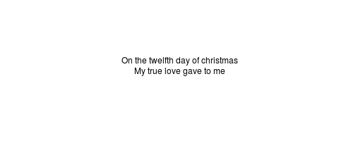
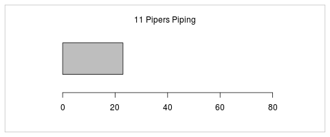
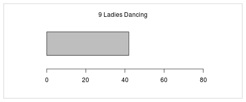
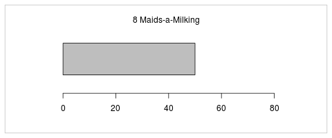
The audio track is the final verse of the song "The Twelve Days of Christmas" sampled from a version by R.Tists for Christmas (CC-BY-NC-SA). The bar plot will be used to show the accumulated number of gifts that "my true love" provides on the 12th day. This example is based on a post on Tumblr by Thomas Levine.
Figure 25, “Some 12 days frames” shows some of the frames that will be used to make up the animation. It starts with a frame containing only text lyrics, then a plot is shown with a bar growing to the right as more gifts are added on each line of the song. The lyrics for each line are shown above the bar.
The timing of the steps in this animation is based on the timing of the audio that will accompany it and the timing of the song varies quite a bit. For example, many of the lyrics are based on three beats (e.g., "four colly birds"), but some are much longer (e.g., "5 golden rings" takes 8 beats), especially the drawn out final line. The following code establishes a vector of lyric lengths.
lengths <- c(rep(3, 7),
             8, # golden rings
             rep(3, 2),
             4, # turtle doves
             17) # partridge
The building blocks of the animation consist of a plot (which draws the x-axis), the lyric text, and the grey bar. We will also make use of a red rectangle to briefly highlight the number of gifts being added for each lyric. The red rectangle appears only for .5 seconds each time, but all of the other components will vary in their duration, so they will take their duration from their container.
background <- atomic(label="bg", durn=NA)
gifttext <- atomic(label="gift", durn=NA)
totalgifts <- atomic(label="cumrect", durn=NA)
numgifts <- atomic(label="hirect", durn=.5)
The text and rectangle building blocks are combined together using a track animation (they run simultaneously). We generate one of these tracks for each line of lyrics, with each track given its own duration.
tracks <- lapply(lengths,
                 function(l) {
                     trac(gifttext, totalgifts, numgifts, durn=l)
                 })
The complete animation has the introductory lyrics first, followed by a track that combines the plot x-axis with a sequence of tracks for each lyric, with everything combined in an overall sequence (see Figure 26, “A 12 days animation sequence”).
introduction <- atomic(label="intro", durn=10)
timeline <- vec(introduction,
                trac(background, do.call("vec", tracks)))
Figure 26. A sequence animation consisting of an atomic animation followed by a track animation that consists of an atomic animation and a sequence of 12 track animations. (animated version)
We will use this animation description to generate timing information for individual frames. For example, the following code produces timing information for frames after 0 seconds, 10 seconds, and 11 seconds, which shows how different animation actions appear in different frames.
frameTiming(timeline)
  label start durn vec    vecNum trac tracNum
1 intro 0     10   Quebec 1
frameTiming(timeline, 10)
  label   start durn vec          vecNum trac         tracNum
1 bg      10    56.0 Quebec       2      Papa         1
2 gift    10     3.0 Quebec:Oscar 2:1    Papa:Charlie 2:1
3 cumrect 10     3.0 Quebec:Oscar 2:1    Papa:Charlie 2:2
4 hirect  10     0.5 Quebec:Oscar 2:1    Papa:Charlie 2:3
frameTiming(timeline, 11)
  label   start durn vec          vecNum trac         tracNum
1 bg      10    56   Quebec       2      Papa         1
2 gift    10     3   Quebec:Oscar 2:1    Papa:Charlie 2:1
3 cumrect 10     3   Quebec:Oscar 2:1    Papa:Charlie 2:2
We now need functions that can make use of the timing information
to draw a frame. These functions contain calls to graphics functions
to draw various components of a frame. For example, the
bg() function sets up a new plot and draws the x-axis.
In some cases, the function needs to use information about the frame.
For example, the gift() function produces a different
text message depending on which iteration of the sequence it is called from.
intro <- function(info) {
    plot.new()
    text(.5, .5,
         "On the twelfth day of christmas\nMy true love gave to me")
}
bg <- function(info) {
    par(mar=c(4, 5, 2, 5), oma=rep(.5, 4))
    plot.new()
    plot.window(c(0, sum(12:1)), c(-.5, 1.5))
    axis(1)
    box("inner", col="grey")
}
gift <- function(info) {
    mtext(gifts[(12:1)[info$vecNum[2]]], side=3)
}
cumrect <- function(info) {
    rect(0, 0, cumsum(12:1)[info$vecNum[2]], 1,
         col="grey")
}
hirect <- function(info) {
    if (info$vecNum[2] == 1) {
        rect(0, 0, 12, 1,
             col="red", border=NA)
    } else {
        rect(cumsum(12:1)[info$vecNum[2] - 1], 0,
             cumsum(12:1)[info$vecNum[2]], 1,
             col="red", border=NA)
    }
}
With these functions defined, an overall function can be created to draw just the components that are active in a frame. This function makes use of the fact that we chose labels for the atomic actions to match the names of the functions that draw the different components of a frame.
drawFrame <- function(info) {
    lapply(info,
           function(x) {
               get(x$label)(x)
           })
}
We can now play the animation by calling
frameApply(). This calls our
drawFrame() function for each of a series
of animation frames. The fps argument
specifies that there should be two frames per second
(which ensures that the highlight rectangles will appear
in at least one frame).
frameApply(timeline, drawFrame, fps=2)
Functions from the animation package can be used to generate an animated movie from this sequence of frames. For producing a movie we use more frames per second to get a smoother result, we do not bother to pause between generating frames, and we use the interval argument to scale the timing so that 1 second in the animation sequence becomes .65 seconds in the movie.
library(animation)

saveVideo(frameApply(timeline, drawFrame, fps=10, pause=FALSE),
          interval=1/10 * .65, ani.height=200,
          outdir="ImageFiles")
The final result, including audio, is available here (requires a web browser with support for the HTML5 <video> element, plus support for the Ogg container format, the Theora video format, and the Vorbis audio format). A GIF version (without audio) is shown in Figure 27, “A 12 days animation”

The complex timing of this animation makes the contribution of
the animaker package more significant in this case.
It is also worth noting that the separation between the overall timing
of the animation and the individual animation actions is again useful,
particularly in this case when it became necessary to repeatedly
experiment with different timings. All that was required was to
change values in the lengths variable and everything
else flowed from that.
This report describes an R package that provides a convenient and flexible way to build descriptions of animation sequences. An animation description can be used to generate a timing scheme that contains information about the start and duration of every action in the animation (or for every frame in the animation).
The main functions in the package are:
atomic()to describe a single step in an animation.vec()to combine animation steps in series.trac()to combine animation steps in parallel.timing()to generate a timing scheme for an animation.
Further functions are provided to manipulate animation descriptions and there are functions for drawing diagrams to help visualise animations descriptions.
This section contains links to the raw R code files. All code is free software, released under the GPL. The animaker package itself is currently only available from github.
The concepts of sequence tracks and sequence animations derive their intellectual ancestry from various systems that can be used to coordinate multimedia resources. These include Microsoft MovieMaker, Microsoft PowerPoint, Adobe Flash, and several javascript libraries: timeline.js, burst-core, and Mozilla's Popcorn.