This report describes an update to the R package 'dvir' to add support for the TikZ graphics package. This allows R users to make use of TikZ drawing capabilities within R graphics.

The 'dvir' package (Murrell, 2020c, Murrell, 2018) provides functions for rendering TeX output on R graphics devices. For example, the following code renders a simple TeX mathematical expression in R graphics.

library(dvir)
grid.latex("$x - \\mu$")

2. Support for TikZ in 'dvir'

TikZ is a TeX package that allows pictures to be drawn within a TeX document. Version 0.3-0 of the 'dvir' package (for R) adds support for TikZ pictures so that we can write TikZ code and have the result rendered in R graphics.

The simplest interface to the new 'dvir' features is via the function grid.tikzpicture. For example, the following code draws (in R) a TikZ picture consisting of two "nodes" connected by a curved line.

grid.tikzpicture("\\path (0, 2) node[circle,draw](x){A} 
                         (4, 0) node[circle,draw](y){B};
                  \\draw (x) .. controls (2, 2) and (2, 0) .. (y);")

The next section describes the full set of new user-level R functions that have been added to the 'dvir' package in version 0.3-0.

3. User interface

The simplest way to render a TikZ picture in R is via the grid.tikzpicture function. This function only requires a character value containing the TikZ code necessary to describe the picture. For example, the following code creates a LaTeX document that consists of just a TikZ picture (and renders the result in R).

grid.tikzpicture("
\\path (0, 0) node[circle,minimum size=.5in,fill=blue!20,draw,thick] (x) {\\sffamily{R}} 
       (3, 0) node[circle,minimum size=.5in,fill=blue!20,draw,thick] (y) {Ti{\\it k}Z!};
\\draw[->] (x) .. controls (1, 1) and (2, 1).. (y);
\\draw[->] (y) .. controls (2, -1) and (1, -1) .. (x);
")

If we want to draw LaTeX content that consists of both normal text and a TikZ picture, we can use the grid.tikz function. This requires that we bracket the TikZ picture with \begin{tikzpicture} and \end{tikzpicture}, but it takes care of loading the TikZ package for us.

grid.tikz("
We can combine normal (\\LaTeX{}) text with a Ti{\\it k}Z picture.
\\begin{tikzpicture}
\\path (0, 0) node[circle,minimum size=.5in,fill=blue!20,draw,thick] (x) {\\sffamily{R}} 
       (3, 0) node[circle,minimum size=.5in,fill=blue!20,draw,thick] (y) {Ti{\\it k}Z!};
\\draw[->] (x) .. controls (1, 1) and (2, 1).. (y);
\\draw[->] (y) .. controls (2, -1) and (1, -1) .. (x);
\\end{tikzpicture}
")

If our TikZ picture makes use of add-on TikZ packages, those must be loaded as well, which means that we must specify the preamble for the TeX code. The grid.tikz and grid.tikzpicture functions use the tikzPreamble and tikzpicturePreamble functions to generate the default preamble.

  \documentclass[12pt]{standalone}
  \def\pgfsysdriver{/usr/local/lib/R/site-library/dvir/tikz/pgfsys-dvir.def}
  \usepackage{tikz}
  
  \begin{document}

Both the tikzPreamble and tikzpicturePreamble functions have a packages argument so that we can specify additional TikZ packages to include in the default preamble. For example, the following preamble loads the decorations.pathmorphing package.

tikzPreamble(packages="decorations.pathmorphing")

  \documentclass[12pt]{standalone}
  \def\pgfsysdriver{/usr/local/lib/R/site-library/dvir/tikz/pgfsys-dvir.def}
  \usepackage{tikz}
  \usetikzlibrary{decorations.pathmorphing}
  \begin{document}

The following code "decorates" the arrows between two labels with a "zigzag" decoration, using the TikZ package decorations.pathmorphing.

grid.tikzpicture("
\\path (0, 0) node[circle,minimum size=.5in,fill=blue!20,draw,thick] (x) {\\sffamily{R}} 
       (3, 0) node[circle,minimum size=.5in,fill=blue!20,draw,thick] (y) {Ti{\\it k}Z!};
\\draw[->, decorate, decoration=zigzag] (x) .. controls (1, 1) and (2, 1).. (y);
\\draw[->, decorate, decoration=zigzag] (y) .. controls (2, -1) and (1, -1) .. (x);
",
    preamble=tikzpicturePreamble(packages="decorations.pathmorphing"))

We can also use the main 'dvir' function grid.latex if, for example, we want to select a different TeX engine. However, in this case we must write an appropriate preamble that loads the TikZ package and specifies the pgfsys-dvir.def driver for TikZ, and we must ensure that the engine uses the tikzSpecial function to handle TeX specials.

The following code draws a combination of normal text plus a TikZ picture using the LuaTeX engine to typeset the content. It also selects a specific font. This requires a preamble that combines the relevant TeX code for the LuaTeX engine with the relevant TeX code for using the TikZ package. (The luaPreamble function can be used to generate a basic preamble for the LuaTeX engine.)

grid.latex("
We can combine normal (\\LaTeX{}) text with a TikZ picture.
\\begin{tikzpicture}
\\path (0, 0) node[circle,minimum size=.5in,fill=blue!20,draw,thick] (x) {\\sffamily{R}} 
       (3, 0) node[circle,minimum size=.5in,fill=blue!20,draw,thick] (y) {TikZ!};
\\draw[->] (x) .. controls (1, 1) and (2, 1).. (y);
\\draw[->] (y) .. controls (2, -1) and (1, -1) .. (x);
\\end{tikzpicture}
",
    preamble=c("\\RequirePackage{luatex85} % For more recent versions of LuaTeX",
               "\\documentclass[12pt]{standalone}",
               "\\usepackage{fontspec}",
               paste0("\\def\\pgfsysdriver{",
                 system.file("tikz", "pgfsys-dvir.def",
                             package="dvir"),
                 "}"),
               "\\usepackage{tikz}",
               "\\setmainfont[Mapping=text-tex]{Lato Light}",
               "\\begin{document}",
               "\\selectfont"),
    engine=luaEngine(special=tikzSpecial))

Once we have this much TeX code it may be more covenient to put the TeX code in a separate file and use the file argument to grid.latex, though we must still ensure that we are using an engine that will process the TikZ specials. The following code produces exactly the same result as the previous code.

grid.latex(file="luaTikz.tex", preamble="", postamble="",
           engine=luaEngine(special=tikzSpecial))

This file-based approach is also more convenient for checking that our TeX code is correct because we can easily process the TeX code outside of R, e.g., by running pdflatex, and checking that result.

4. Integrating R graphics and TikZ graphics

Almost all of the examples so far have only consisted of a TikZ picture by itself. This section looks at the issue of combining a TikZ picture with other R graphics output.

By default, the 'dvir' package draws TeX output within a 'grid' viewport that is based on the bounding box of the TeX output and, by default, the TeX output is drawn in the centre of the current viewport.

For example, the following code draws a 'lattice' plot (Sarkar, 2008), navigates to the plot region viewport, and draws a label using grid.latex. The result is that the label is drawn in the centre of the 'lattice' plot region (a grey rectangle is drawn to show the extent of the bounding box of the TikZ output).

library(lattice)
xyplot(mpg ~ disp, mtcars)
downViewport("plot_01.panel.1.1.vp")
grid.latex("Toyota Corolla")
downViewport("dvi.vp")
grid.rect(gp=gpar(col="grey", fill=NA))

It is possible to explicitly position the TeX output and it is possible to specify an explicit justification. For example, the following code draws the TeX label just above and to the right of the relevant data point in the 'lattice' plot.

corolla <- mtcars[grep("Toyota", rownames(mtcars))[1],]
xyplot(mpg ~ disp, mtcars)
downViewport("plot_01.panel.1.1.vp")
grid.points(corolla$disp, corolla$mpg, pch=16, gp=gpar(col="#0080ff"))
grid.latex(rownames(corolla),
           x=unit(corolla$disp, "native") + unit(2, "mm"),
           y=unit(corolla$mpg, "native") + unit(2, "mm"),
           just=c("left", "bottom"))
downViewport("dvi.vp")
grid.rect(gp=gpar(col="grey", fill=NA))

The next example demonstrates a more difficult task. In this case, we are drawing a TikZ picture that consists of a label plus two curves from the label to two data points within the plot.

toyota <- mtcars[grep("Toyota", rownames(mtcars)),]
xyplot(mpg ~ disp, mtcars)
downViewport("plot_01.panel.1.1.vp")
grid.points(toyota$disp, toyota$mpg, pch=16, gp=gpar(col="#0080ff"))
toyotaX <- convertX(unit(toyota$disp, "native"), "cm", valueOnly=TRUE)
toyotaY <- convertY(unit(toyota$mpg, "native"), "cm", valueOnly=TRUE)
path <- paste(c(paste0("\\draw[->] (a) .. ",
                       "controls +(left:2cm) and +(right:2cm) .. ",
                       "(", toyotaX[1] + .2, ",", toyotaY[1], ");"),
                paste0("\\draw[->] (a) .. ",
                       "controls +(left:2cm) and +(right:2cm) .. ",
                       "(", toyotaX[2] + .2, ",", toyotaY[2], ");")),
               sep="\n")
picture <- paste(c(paste0("\\path (", toyotaX[1] + 7, ",", toyotaY[1] - 2, ") ",
                          "node (a) {Toyotas};"),
                   path),
                 sep="\n")
grid.tikzpicture(picture,
                 bbox=c(0, 0,
                        convertWidth(unit(1, "npc"), "cm", valueOnly=TRUE),
                        convertHeight(unit(1, "npc"), "cm", valueOnly=TRUE)))
downViewport("dvi.vp")
grid.rect(gp=gpar(col="red", fill=NA))

The challenge here is to align the coordinate system of the TikZ picture with the 'grid' coordinate systems in R. There are several points to make about the code above:

By specifying bbox in a call to grid.tikzpicture, we are inserting a small piece of TikZ code at the end of the TikZ picture, like that shown below.

dvir:::tikzBBox(0, 0, 1, 1)

  [1] "\\pgfresetboundingbox\\useasboundingbox (0,0) rectangle (1,1);"

We can also insert code like that at any point in our TikZ code in order to control the bounding box of the TikZ picture. The \useasboundingbox command will intersect the specified rectangle with the current bounding box of the picture (which can only make the bounding box smaller). The \pgfresetboundingbox command resets the bounding box of the picture (so we can make the bounding box larger).

As an example, the following code reproduces the previous example, but in this case, instead of using the bbox argument to grid.tikzpicture, we include \useasboundingbox in the TikZ code. (This code also does NOT include the text label, it just draws the lines and arrows, for reasons that will become clearer shortly.) The idea with this approach is that we set the bounding box of the TikZ picture to match the range of x/y values of the two data points that we are drawing lines to and then we position the TikZ picture within R with its top-left corner at the top-left of the two data points. A red rectangle has been added to show the TikZ picture bounding box that we enforced (and its location on the plot).

xyplot(mpg ~ disp, mtcars)
downViewport("plot_01.panel.1.1.vp")
grid.points(toyota$disp, toyota$mpg, pch=16, gp=gpar(col="#0080ff"))
picture <- paste(c(paste0("\\path (", toyotaX[1] + 7, ",", toyotaY[1] - 2, ") ",
                          "node (a) {};"),
                   path,
                   paste0("\\pgfresetboundingbox\\useasboundingbox (",
                          toyotaX[1], ",", toyotaY[1], ") rectangle (",
                          toyotaX[2], ",", toyotaY[2], ");")),
                 sep="\n")
grid.tikzpicture(picture,
                 x=unit(toyotaX[1], "cm"), y=unit(toyotaY[1], "cm"),
                 just=c("left", "top"))
downViewport("dvi.vp")
grid.rect(gp=gpar(col="red", fill=NA))

One caveat with this approach (explicitly controlling the bounding box of the TikZ picture) is that it only works for the TikZ picture AND it only works for non-text elements of the TikZ picture. Any text, either within the TikZ picture or outside it, will expand the bounding box of the overall TeX drawing. The following code demonstrates this by adding the text label back into the TikZ picture. We enforce a bounding box on the non-text elements of the picture, but the text label expands the right side of the bounding box to include the label. The result is still aligned correctly in this case, but more by good fortune than good planning.

xyplot(mpg ~ disp, mtcars)
downViewport("plot_01.panel.1.1.vp")
grid.points(toyota$disp, toyota$mpg, pch=16, gp=gpar(col="#0080ff"))
picture <- paste(c(paste0("\\path (", toyotaX[1] + 7, ",", toyotaY[1] - 2, ") ",
                          "node (a) {Toyotas};"),
                   path,
                   paste0("\\pgfresetboundingbox\\useasboundingbox (",
                          toyotaX[1], ",", toyotaY[1], ") rectangle (",
                          toyotaX[2], ",", toyotaY[2], ");")),
                 sep="\n")
grid.tikzpicture(picture,
                 x=unit(toyotaX[1], "cm"), y=unit(toyotaY[1], "cm"),
                 just=c("left", "top"))
downViewport("dvi.vp")
grid.rect(gp=gpar(col="red", fill=NA))

The 'ggplot2' example

This section outlines the steps required to produce the 'ggplot2' example in the Section on Support for TikZ in 'dvir'. This demonstrates a more complex example of integrating R graphics and TikZ graphics.

temps <- read.table("graph.txt", skip=5, header=FALSE,
                    col.names=c("year", "temp", "smooth"))

ggplot(temps) +
    geom_line(aes(x=year, y=temp)) +
    geom_smooth(aes(x=year, y=temp), se=FALSE,
                colour=adjustcolor(1, alpha=.5), lwd=3)

We are going to visit the 'grid' viewports that were used to draw the 'ggplot2' plot so a preliminary step is to "force" the 'ggplot2' plot so that we have access to its viewports (and grobs).

downViewport("panel.7-5-7-5")

We identify and extract the 'grid' grob corresponding to the smoothed line. This is the second polyline in the plot; the first polyline is the jagged line representing the raw temperature values.

smooth <- grid.grep("GRID.polyline", grep=TRUE, global=TRUE)[[2]]
smoothGrob <- grid.get(smooth)

This gives us access to the x/y coordinates of the smoothed line and we use those to generate a TikZ path description that corresponds to the smoothed line on the plot (in centimetres).

path <- paste(paste0("(",
                     round(convertX(smoothGrob$x, "cm", valueOnly=TRUE), 2),
                     ",",
                     round(convertY(smoothGrob$y, "cm", valueOnly=TRUE), 2),
                     ")"),
              collapse=paste0("-", "-"))

  \draw[->] (a) .. controls +(left:2cm) and +(right:2cm) .. (0 \draw[->] (a) .. controls +(left:2cm) and +(right:2cm) .. (2 ...

Now we can call grid.tikzpicture to draw that path and "decorate" the path with a text label: "the warming planet". Note that we generate a preamble that loads the required decorations.text package and we specify a bounding box for the TikZ picture that corresponds to the current viewport.

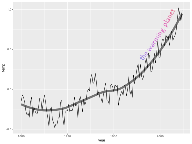
grid.tikzpicture(paste("\\draw[postaction={decorate, decoration={raise=8mm, text along path,text={|\\sffamily\\Huge|the warming planet},text align=right}}] ",
                       path,
                       ";"),
                 preamble=tikzpicturePreamble(packages="decorations.text"),
                 bbox=c(0, 0,
                        convertWidth(unit(1, "npc"), "cm", valueOnly=TRUE),
                        convertHeight(unit(1, "npc"), "cm", valueOnly=TRUE)))

At this point, we have the original 'ggplot2' plot with a TikZ path and text decoration on top (note the thin black TikZ path on top of the thick translucent 'ggplot2' smoother).

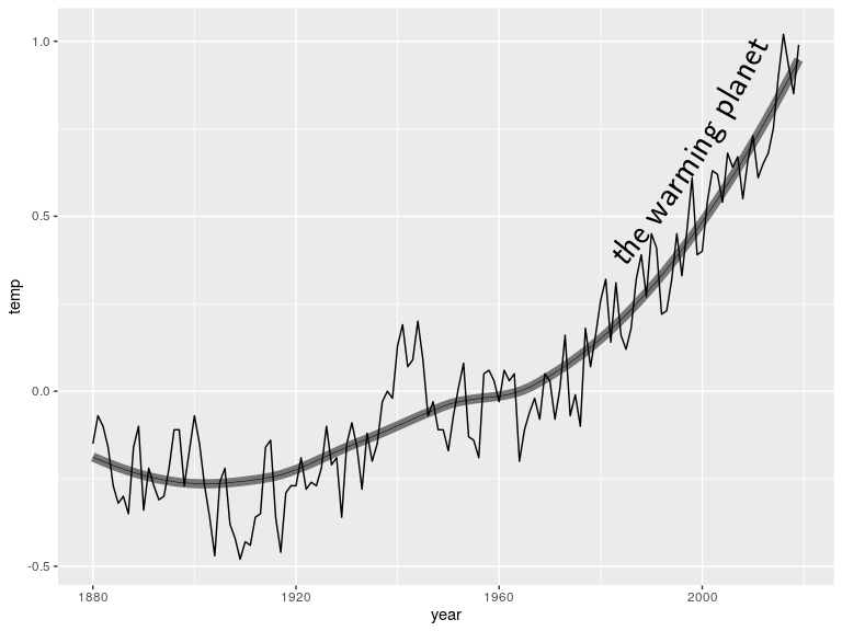
We now have 'grid' graphics in R to work with, so we can do things like removing the TikZ path to just leave the text decoration ...

grid.remove("DVIgrob::gTree::polyline", grep=TRUE)

tikzText <- grid.grep("DVIgrob::gTree::text", grep=TRUE, global=TRUE)
cols <- hcl(seq(270, 360, length.out=length(tikzText)), 80, 60)
for (i in seq_along(tikzText)) {
    grid.edit(tikzText[[i]], gp=gpar(col=cols[i]), redraw=FALSE)
}
grid.refresh()

5. How it works

This section describes the internal design of the TikZ support in the 'dvir' package.

The 'dvir' package provides some light wrappers around calls to the TeX engine to process TeX documents and generate DVI output. The more important work done by the 'dvir' package is reading the DVI output and calling the 'grid' graphics system to render the result.

Generating DVI output

A DVI file consists mainly of a set of instructions that select a font, define a location, then specify a character to draw. For example, the output below is the DVI output that corresponds to the simple mathematical expression from the very first example in this report.

  pre          version=2, num=25400000, den=473628672, mag=1000,
               comment= TeX output 2020.11.24:2202
  bop          counters=1 0 0 0 0 0 0 0 0 0, p=-1
  down4        a=1069005536
  push
  y4           a=-1073741823 
  down4        a=1073741823
  push
  right3       b=-4736287
  y0 
  xxx1         k=30
               x=papersize=23.96289pt,7.77777pt
  xxx1         k=49
               x=ps::%%HiResBoundingBox: 0 0 23.96289pt 7.77777pt.
  down3        a=509724
  push
  push
  push
  down3        a=-127431
  fnt_def_1    fontnum=10, checksum=195060286, scale=655360, design=655360,
               fontname=cmmi10
  fnt_num_10
  set_char_120 'x'
  w3           b=145632 
  fnt_def_1    fontnum=13, checksum=555887770, scale=655360, design=655360,
               fontname=cmsy10
  fnt_num_13
  set_char_0   ''
  w0 
  fnt_num_10
  set_char_22  ''
  pop
  pop
  pop
  pop
  pop
  eop
  post
  fnt_def_1    fontnum=13, checksum=555887770, scale=655360, design=655360,
               fontname=cmsy10
  fnt_def_1    fontnum=10, checksum=195060286, scale=655360, design=655360,
               fontname=cmmi10
  post_post

The DVI output above contains operations like down4 and right3 to define the location, fnt_def_1 to define a font, fnt_num_10 to select a font, and set_char_120 to draw an 'x'.

How are TikZ graphics expressed in DVI output? The following output shows a very simple example for a TikZ picture that just draws a straight line, like the image below.

  xxx1         k=11
               x=ps::[begin]
  xxx1         k=9
               x=ps:: pgfo
  xxx1         k=10
               x=ps:: save 
  xxx1         k=15
               x=ps:: 0 setgray 
  xxx1         k=17
               x=ps:: 0.3985 pgfw 
  push
  xxx1         k=10
               x=ps:: save 
  xxx1         k=20
               x=ps:: 0.0 0.0 moveto 
  xxx1         k=28
               x=ps:: 28.3468 28.3468 lineto 
  xxx1         k=12
               x=ps:: pgfstr 
  xxx1         k=13
               x=ps:: restore 
  pop
  xxx1         k=13
               x=ps:: newpath 
  xxx1         k=13
               x=ps:: restore 
  xxx1         k=9
               x=ps:: pgfc
  xxx1         k=9
               x=ps::[end]

The main point is that TikZ pictures become "special" operations in DVI output (xxx1).

The special operations describe how to draw the straight line. There are operations to set the drawing color (setgray), set the line width (pgfw), define a "path" (moveto and lineto), and "stroke" the path (pgfstr).

Anyone familiar with the PostScript language (Adobe Systems Inc., 1999), will recognise the content of the TikZ special operations as PostScript commands. By default (when using latex as the TeX engine), TikZ produces PostScript commands in DVI output.

It is possible to generate DVI output with TikZ pictures represented by commands in other languages. For example, the DVI below is for the same TikZ path, but by selecting the pgfsys-dvisvgm.def "driver", it produces SVG in the DVI output. Again, we only show the relevant part of the DVI output.

  xxx1         k=60
               x=dvisvgm:raw <g transform="translate({?x},{?y}) scale(1,-1)">
  xxx1         k=21
               x=dvisvgm:raw <g>{?nl} 
  xxx1         k=50
               x=dvisvgm:raw <g stroke="rgb(0.0%,0.0%,0.0%)">{?nl} 
  xxx1         k=48
               x=dvisvgm:raw <g fill="rgb(0.0%,0.0%,0.0%)">{?nl} 
  xxx1         k=42
               x=dvisvgm:raw <g stroke-width="0.4pt">{?nl} 
  push
  xxx1         k=21
               x=dvisvgm:raw <g>{?nl} 
  xxx1         k=22
               x=dvisvgm:raw <path d=" 
  xxx1         k=45
               x=dvisvgm:raw M  0.0 0.0 L  28.45274 28.45274  
  xxx1         k=39
               x=dvisvgm:raw " style="fill:none"/>{?nl} 
  xxx1         k=22
               x=dvisvgm:raw </g>{?nl} 
  pop
  xxx1         k=22
               x=dvisvgm:raw </g>{?nl} 
  xxx1         k=22
               x=dvisvgm:raw </g>{?nl} 
  xxx1         k=22
               x=dvisvgm:raw </g>{?nl} 
  xxx1         k=22
               x=dvisvgm:raw </g>{?nl} 
  xxx1         k=16
               x=dvisvgm:raw </g>

Even better, it is possible to write a custom TikZ driver so that we can control the TikZ commands in DVI output. The 'dvir' package includes a pgfsys-dvir.def file that defines such a driver and this driver is selected by default by the functions grid.tikzpicture, grid.tikz, and tikzPreamble. An example of the DVI output from this driver is shown below, again just for the simple straight line TikZ picture (note the dvir:: prefixes).

  xxx1         k=21
               x=dvir:: begin-picture;
  xxx1         k=21
               x=dvir:: begin-scope ; 
  push
  right3       b=655359
  xxx1         k=56
               x=dvir:: begin-scope col=gray(0) fill=gray(0) lwd=0.4pt ; 
  xxx1         k=18
               x=dvir:: new-path ; 
  xxx1         k=49
               x=dvir:: moveto 0.0,0.0:lineto 28.45274,28.45274:; 
  xxx1         k=15
               x=dvir:: stroke; 
  xxx1         k=18
               x=dvir:: end-scope; 
  pop
  right3       b=655359
  xxx1         k=18
               x=dvir:: end-scope; 
  xxx1         k=55
               x=dvir:: end-picture -0.2pt,-0.2pt,28.65274pt,28.65274pt;

Now that we can control the representation of TikZ pictures in DVI output, the 'dvir' package is essentially able to "talk to itself"; it knows what the TikZ output will look like because it wrote the TikZ output.

The TeXengine function has a new special argument so that we can specify how DVI special operations should be handled. By default, this argument is noSpecial which means that DVI specials are ignored. If we specify special=tikzSpecial, then TikZ specials are converted to 'grid' drawing (as described in the next section). The grid.tikzpicture and grid.tikz functions use an engine that uses tikzSpecial by default.

Converting DVI output to 'grid' grobs

If we look closer at the DVI output above, we can see that the DVI content that represents the TikZ picture has the following structure:

This render-off-screen-then-capture approach is also applied to standard DVI output, which is a change from previous versions of 'dvir'. In previous versions, 'grid' grobs were generated from each DVI operation and accumulated in a final gTree. Now, each DVI operation produces drawing (off-screen) and then a grid.grab generates the final gTree.

A further complication arises when a TikZ picture contains text labels like the image below.

  xxx1         k=21
               x=dvir:: begin-picture;
  xxx1         k=21
               x=dvir:: begin-scope ; 
  push
  right3       b=655359
  xxx1         k=56
               x=dvir:: begin-scope col=gray(0) fill=gray(0) lwd=0.4pt ; 
  xxx1         k=18
               x=dvir:: new-path ; 
  xxx1         k=49
               x=dvir:: moveto 0.0,0.0:lineto 28.45274,28.45274:; 
  xxx1         k=15
               x=dvir:: stroke; 
  push
  push
  xxx1         k=21
               x=dvir:: begin-scope ; 
  xxx1         k=21
               x=dvir:: begin-scope ; 
  xxx1         k=52
               x=dvir:: transform 1.0,0.0,0.0,1.0,25.95274,-2.15277; 
  push
  fnt_def_1    fontnum=7, checksum=1274110073, scale=655360, design=655360,
               fontname=cmr10
  fnt_num_7
  set_char_97  'a'
  pop
  xxx1         k=18
               x=dvir:: end-scope; 
  xxx1         k=18
               x=dvir:: end-scope; 
  pop
  pop
  xxx1         k=18
               x=dvir:: end-scope; 
  pop
  right3       b=655359
  xxx1         k=18
               x=dvir:: end-scope; 
  xxx1         k=59
               x=dvir:: end-picture -0.2pt,-5.48575pt,34.28572pt,28.65274pt;

The label is recorded as a standard DVI set_char, but it is positioned by a special transform. A TikZ picture can also generate transform output for so-called "protocolled" picture elements (e.g., arrow heads). For every transform, we push a new 'grid' viewport to position the 'grid' drawing appropriately. The viewports generated by transform specials are popped again at the next end-scope.

Metric calculations

The above description applies to the "rendering" sweep through the DVI content. That is preceded by a font sweep (to process all font definitions in the DVI content) and a metric sweep (to determine the bounding box for the DVI content). No action is taken for special (TikZ) DVI content during the font sweep.

The metric sweep is relatively straightforward, mostly consisting of simply reading the bounding box information from the end-picture. The only complication is from text labels within a TikZ picture. The metric sweep also maintains a stack of transforms so that the overall DVI bounding box is calculated correctly for these text labels.

6. Discussion

Version 0.3-0 of the 'dvir' package includes support for TikZ pictures within a TeX document. This allows us to make use of the graphics capabilites of TikZ to draw images in R. TikZ's graphics capabilities are quite extensive (its manual runs to over 1300 pages), including sophisticated path construction, three-dimensional drawings, ERD diagrams, data visualisations, and much more.

The idea behind adding TikZ support to 'dvir' is that we get access to all of TikZ's capabilities in one swoop. By allowing R to understand TikZ output (in DVI files), we can render any TikZ picture as part of an R image (though see the section on limitations below).

The 'tikzDevice' package

The most obvious alternative to 'dvir' is the 'tikzDevice' package (Sharpsteen and Bracken, 2020). This provides an R graphics device that converts R's graphical output to TikZ pictures; essentially the inverse of what 'dvir' does. The end result is similar in that we have a combination of R graphics capabilities and TikZ capabilities.

The difference is that, with 'tikDevice', we start in R, generate an image, export it to a TikZ picture and we end up with TeX code that we can embed in (and potentially integrate with) a TeX document. We end up in the TeX world.

With 'dvir', we start in R, generate a TikZ picture (TeX code), convert that to DVI, then import (and integrate) the result back into R. We end up in the R world.

Each option has advantages for different scenarios, or at least for different stages in a visualisation project. Ending up in R is possibly more useful when we are in the process of building a data visualisation. It may be easier to add and combine further drawing. Ending up in TeX is a good place to be when we want to incorporate a data visualisation within a larger document like a report or book.

It is also possible to use 'tikzDevice' and 'dvir' in concert. We could make use of 'tikzDevice' to help generate TikZ code (e.g., using tikz(console=TRUE, bareBones=TRUE)) and an R image that we export to TeX via 'tikzDevice' could conceivably include R graphics output that contains elements that were generated by 'dvir' (from TikZ code).

Other approaches

An alternative approach to providing TikZ-like graphics capabilities is to reimplement those capabilities in R. For example, the 'plotrix' package (Lemon, 2006) has an arctext function for drawing text along an arc of a circle. Many other packages, like 'ggforce' (Pedersen, 2020b), add various drawing capabilities. The advantage of 'dvir' is that we can access all of TikZ without having to reimplement any of it.

This does not remove the need for R packages that implement new graphics features. There are R packages that add capabilities that are not (easily) available in TikZ, like 'vwline' (Murrell, 2019). Furthermore, the 'dvir' package only works on specific R graphics devices, so there is value in R packages that work across all graphics devices. Finally, R packages that implement a feature similar to a TikZ capability are unlikely to overlap precisely with the TikZ capability, with features missing on either side.

Limitations of 'dvir'

In addition to the existing limitations of 'dvir' (such as support only being available for PDF and Cairo devices), there are some limits on the TikZ support within 'dvir'.

TikZ (and the underlying PGF system) allow the user to control the coordinate system within which drawing occurs. At the time of writing, the 'dvir' package assumes that locations within TikZ code are in the default coordinate system of centimetres. It also assumes that the values in TikZ's DVI output are in millimetres (unless they carry an explicit unit). This is vulnerable to internal changes to TikZ and possibly to the user writing TikZ code in a different coordinate system.

The underlying PGF system also allows more complex control of coordinate systems, including a "canvas transform" that can include scaling and shearing transformations (in addition to translation and rotation). The 'dvir' package can currently only cope with this canvas transform as long as it only involves translation and/or rotation. This means that some TikZ pictures will not be drawn correctly. On the other hand, the PGF/TikZ manual provides stern warnings about using the canvas transformation matrix, so hopefully this limitation will not be encountered very often.

Another difficulty with the TikZ support in 'dvir' is that the R user has to write raw TikZ code. This is both unfamiliar code for an R user and the flexible, somewhat natural-language syntax that TikZ allows, can be difficult to absorb. This leads us nicely on to the next section on future work.

Future work

The TikZ support in 'dvir' is not yet complete. For example, clipping, gradient fills, and pattern fills are not yet supported. With the improved support for these features in the R graphics engine for R 4.1.0 (Murrell, 2020b), adding these capabilites to 'dvir' should be possible in the future.

As pointed out in the previous section, writing raw TikZ may not be the easiest task for an R user. This suggests that there might be value in an R function interface to generating TikZ code. As we can see with functions like tikzPreamble, it can be useful to have R functions that help to generate TeX code (and it is straightforward to write such functions). Such TeX-generating R functions already exist in several packages, e.g., 'xtable' (Dahl et al., 2019), but an R interface to TikZ graphics would be an interesting addition (and an interesting challenge).

The TikZ package is just one way to draw graphics in the TeX world. There may be opportunities to support other TeX-based graphics systems by adding support in 'dvir' for other sets of DVI specials. Unfortunately, support for one major alternative, PStricks (Van Zandt, 2007), does not make sense because PStricks produces DVI specials that are specifically designed for PostScript output. It does not have the concept of multiple backends like TikZ does. Importing DVI with PStricks specials could possibly be achieved by capturing chunks of PostScript output within DVI using the 'grImport' package (Murrell, 2009), but a better approach would be just to generate PostScript from the whole TeX file and 'grImport' that entire PostScript file (although that may require improvements to the font import facilities in 'grImport').

7. Technical requirements

The examples and discussion in this document relate to version 0.3-0 of the 'dvir' package.

This report was generated within a Docker container (see the Resources section below).

8. Resources

How to cite this document

Murrell, P. (2020). "Adding TikZ support to 'dvir'" Technical Report 2020-05, Department of Statistics, The University of Auckland. version 1. [ bib | DOI | http ]

Adding TikZ support to 'dvir'

Table of Contents:

1. Introduction