Variable Fonts in R Graphics

This document describes the addition of support for variable fonts in R, when rendering glyphs, plus changes to the CRAN package xdvir to take advantage of that new support, when rendering LaTeX fragments.

1. Introduction

Since R version 4.3.0 (R Core Team, 2025), it has been possible to render text from a set of typeset glyph information, using functions grDevices::glyphFont() to specify a font, grDevices::grid.glyphInfo() to specify glyphs within the font and a position for each glyph, and grid::grid.glyph() to do the drawing. For example, the following code draws the letter "t" (glyph number 409) from (a local copy of) the Google font Recursive.

fontpath <- file.path(getwd(), "Fonts", "Recursive-VariableFont.ttf")

font <- glyphFont(fontpath, 0, "Recursive", 400, "normal", PSname="Recursive")
info <- glyphInfo(id=409, x=0, y=0, font=1, size=10,
                  fontList=glyphFontList(font), width=8, height=12)
grid.newpage()
grid.glyph(info)

In the development version of R, to become version 4.6.0, support has been added for using variable fonts when rendering glyphs. This comes in the form of a new argument called variations for the grDevices::glyphFont() function, which allows variations on a font to be specified. For example, the following code draws the letter "t" using the Recursive font, as before, but this time specifies a very bold variation of the font. The variation wght=900 means a weight of 900 (out of 1000). For comparison, a normal font weight is typically 400 and a bold font weight is typically 700.

boldFont <- glyphFont(fontpath, 0, "Recursive", 400, "normal", PSname="Recursive",
                      variations=c(wght=900))
info <- glyphInfo(id=409, x=0, y=0, font=1, size=10,
                  fontList=glyphFontList(boldFont), width=8, height=12)
grid.newpage()
grid.glyph(info)

This means that it is now possible to make use of variable fonts when drawing text in R graphics (in the development version of R), although, at the time of writing, support is limited to Cairo-based graphics devices (except for cairo_pdf()) and the quartz() graphics device.

However, we may be left wondering what we could use variable fonts for and how we might use them without specifying every single glyph and every single glyph position for the text that we want to draw.

This report explains what variable fonts are, demonstrates new features in the xdvir package that allow users to make use of variable fonts when drawing text in R graphics, and provides an example use of variable fonts in statistical plots.

2. Variable fonts

Most fonts are available in multiple variations, such as italic or bold, but usually each variation is provided as a separate font file. For example, on the system used to build this report, there are four variations on the NotoSans font in four separate files:

A variable font is different because it effectively contains different font variations within a single font file (and allows for many more variations). The font provides a set of axes and we are able to select different values for each axis to produce variations on the font.

In addition, it is possible for a font to have a custom axis, which could be called anything (as long as it is four ASCII letters, all capitals) and could take any value (as long as it is a number).

For example, the Recursive font that we have been using has the standard wght axis that allows a wide range of font weights and a custom CASL axis that takes the values 1 or 0 and allows for a "casual" font style (or not).

3. Rendering glyphs with xdvir

Using grid.glyph() directly, as demonstrated in the Introduction, is difficult because of the need to specify a font by file name and each glyph within the font by number, along with precise locations for each glyph. It is easier to use a package that figures out font file names, glyph numbers and positions for us. One example is the xdvir package (Murrell, 2025b), which can render LaTeX fragments (with glyph rendering under the hood). For example, the following code draws the letter "t" using the Recursive font, just like in the first example of the Introduction, but with much less detail required from the user.

grid.newpage()
grid.latex("t",
           packages=fontspecPackage(font=fontpath),
           gp=NULL)

4. Variable fonts in xdvir

Version 0.2-0 of the xdvir package has added support for variable fonts (in LaTeX fragements). This takes two forms: first of all, there are new arguments to the fontspecPackage() function that help with generating LaTeX fragments that make use of variable fonts; and secondly, there is a new "luahbtex" TeX engine that can comprehend the DVI output that is generated from LaTeX code that makes use of variable fonts. For details about LaTeX packages and TeX engines in the xdvir package, see Murrell, 2025a.

For example, the following code draws the letter "t" using the Recursive font with a weight of 900. In order to set the font weight to 900, it is necessary not only to specify axes=c(wght=900), but also to specify renderer="harfbuzz", so that the variable font axis information is recorded in the DVI output, and engine="luahbtex", so that the DVI output is read into R correctly. It is also necessary to have a recent lualatex version with variable font support (1.17.0 at least).

grid.newpage()
grid.latex("t",
           packages=fontspecPackage(font=fontpath,
                                    renderer="harfbuzz",
                                    axes=c(wght=900)),
           gp=NULL,
           engine="luahbtex")

The next example demonstrates more complex control over the use of a variable font. In this case, instead of setting up an overall font weight for a very simple LaTeX fragment, we have a more complex LaTeX fragment that specifies separate font weights for separate words.

grid.newpage()
grid.latex(r"(
\addfontfeature{RawFeature={axis={wght=100}}}light
\addfontfeature{RawFeature={axis={wght=500}}}medium
\addfontfeature{RawFeature={axis={wght=900}}}dark
)",
           packages=fontspecPackage(font=fontpath,
                                    renderer="harfbuzz"),
           gp=NULL,
           engine="luahbtex")

Although the example above requires more complex LaTeX code, that code can easily be generated programmatically using basic tools, as demonstrated in the addWeight() function below.

addWeight <- function(label, weight) {
    paste0(r"(\addfontfeature{RawFeature={axis={wght=)",
           weight, "}}}", label)
}
addWeight(c("light", "medium", "dark"),
          c(100, 500, 900))

  [1] "\\addfontfeature{RawFeature={axis={wght=100}}}light" 
  [2] "\\addfontfeature{RawFeature={axis={wght=500}}}medium"
  [3] "\\addfontfeature{RawFeature={axis={wght=900}}}dark"

5. Variable fonts in plots

Being able to specify axes for variable fonts is interesting and fun, but does it have any application to statistical graphics?

Brath and Banissi, 2017 propose that we can treat font weight as a visual channel that can be used to encode data values, just like the standard visual channels of position, length, colour, etc. For example, we can encode data values as the weight of text labels.

As a demonstration of this idea, very loosely based on Brath and Banissi, 2017 Figure 21, we will first produce a choropleth map, which encodes data values as the fill colour of map regions, then we will produce an alternative map that encodes data values as the weights of region labels.

The following code uses the sf (Pebesma, 2018) and dplyr (Wickham et al., 2023) packages to set up the data for the map. This consists of youth crime rates (offenders per 10,000 population) in each police district of New Zealand for 2021 (from the Youth Justice Indicator Report 2021).

library(sf)
library(dplyr)
crimeDistrict <- read.csv("YouthCrime/crime-district.csv") |>
    ## For joining with map data
    mutate(district = gsub("Bay Of Plenty", "Bay of Plenty",
                           gsub("Counties Manukau", "Counties/Manukau",
                                district)))
crimeDistrict <- subset(crimeDistrict,
                        year == 2021,
                        district != "Outside New Zealand (District)")
crimeDistrict$yearDate <- as.Date(paste0(crimeDistrict$year, "-06-30"))
districts <-
    st_read("SHP/nz-police-district-boundaries-29-april-2021.shp",
            quiet=TRUE)
## Drop unnecessary Z dimension from some geometries
districts <- st_zm(districts)
centroids <- st_coordinates(st_centroid(st_geometry(districts)))
districts$X <- centroids[,1]
districts$Y <- centroids[,2]
districts <- inner_join(districts, subset(crimeDistrict, year == 2021),
                        by=join_by(D_MACRON == district))

The following code sets up a ggplot2 plot (Wickham, 2016) with the common aspects of the map. This will allow us to more easily see how the code differs from a choropleth map to the label weight version.

library(ggplot2)
gg <- ggplot() +
    scale_fill_continuous(name="crime rate", high="#132B43", low="#56B1F7") +
    coord_sf(expand=FALSE) +
    xlab(NULL) +
    ylab(NULL) +
    ggtitle("Youth Crime in New Zealand",
            "Distinct offenders per 10,000 pop.") +
    theme_minimal() +
    theme(plot.margin=margin(20, 0, 20, 0),
          axis.ticks=element_blank(),
          axis.text=element_blank(),
          panel.grid=element_blank(),
          legend.position="inside",
          legend.position.inside=c(1, 0),
          legend.justification=c(1, 0),
          legend.margin=margin(0))

The following code generates a choropleth map that maps crime rate to the fill colour for each police district. The darker regions represent higher crime rates.

gg + geom_sf(data=districts, aes(fill=rate), colour="white", linewidth=.6) +
     coord_sf(expand=FALSE)

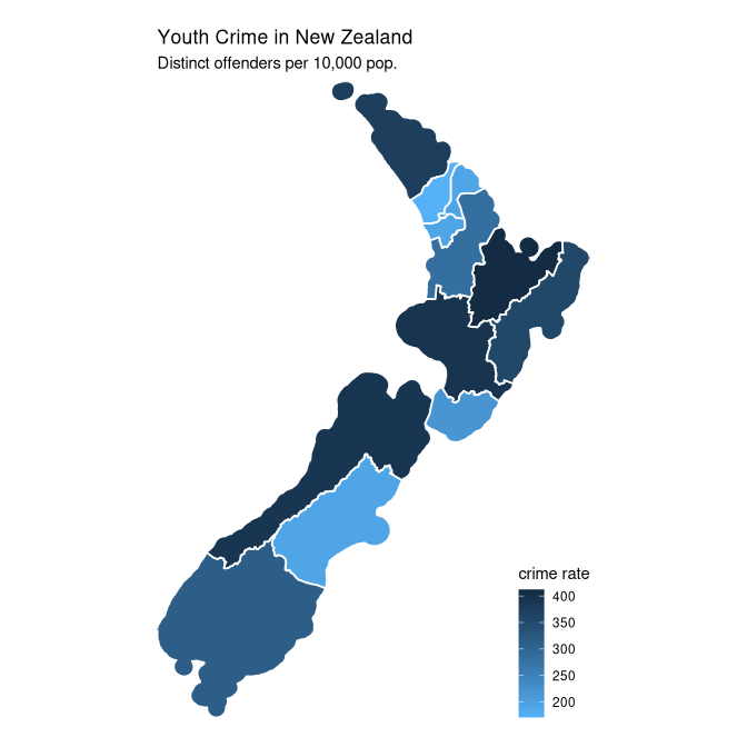
The benefit of using a map like this is that we (Kiwis) can easily decode the geographic locations of different police districts because the shapes are familiar.

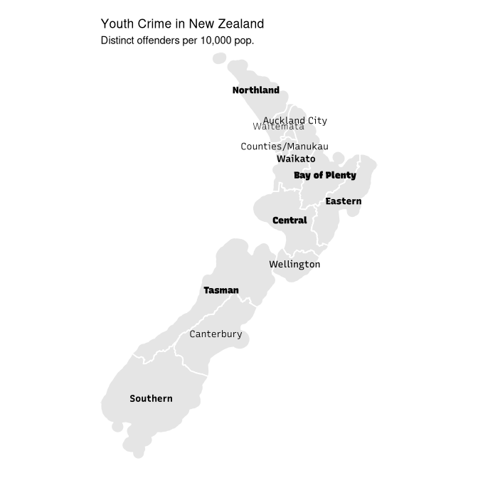
One problem with a choropleth map like this is that the police districts differ in terms of size and shape as well as in terms of fill colour. This complicates the comparison of crime rates between police districts because the map regions differ in terms of fill colour and size and shape. Ideally, in order to effectively compare crime rates between police districts, the map regions would differ only in terms of fill colour (and position). This provides a motivation for an alternative encoding that does not rely on the size and shape of each police district.

We will develop an alternative map that encodes crime rate as the weight of text labels.

The first step is to transform the crime rate to a range of font weights. In the case of the Recursive font, valid weights range from 300 to 1000.

districts$rateStd <- 300 +
                     700 * (districts$rate - min(districts$rate)) /
                            diff(range(districts$rate))

There is a geom_latex() in the xdvir package, but it does not provide the flexibility that we require to select a local font file, so we will add text labels to each police district using the gggrid package (Murrell, 2022). The following code sets up a function to generate the police district labels as grid grobs that will draw LaTeX fragments. We make use of the addWeight() function from above to generate the LaTeX code that controls the font weight for each label.

library(gggrid)
labelTeX <- function(data, coords) {
    label <- data$label
    tex <- addWeight(label, round(data$weight))
    latexGrob(tex, coords$x, coords$y,
              packages=fontspecPackage(font=fontpath,
                                       renderer="harfbuzz"),
              engine="luahbtex",
              gp=NULL)
}

The following code draws the alternative map. We draw police districts as before, but this time they are all filled with the same (light grey) colour. A label is added for each police district with the crime rate encoded as the weight of the label. Bolder labels reflect higher crime rates.

With this map, we can still see the location of each police district, but now the crime rates are more easily compared because different crime rates are encoded simply as the font weights of the police district labels. It is also easier (even for non-Kiwis) to identify the different police districts because they are now all labelled.

gg + geom_sf(data=districts, fill="grey90", colour="white", linewidth=.6)  +
     coord_sf(expand=FALSE) +
     grid_panel(data=districts, labelTeX, aes(X, Y, label=D_MACRON,
                weight=rateStd))

6. Acknowledgements

The original suggestion to add support for variable fonts came from Thomas Lin Pedersen, the author of the marquee package (Pedersen and Mitáš, 2025), among many other things. The marquee package is similar to xdvir in that it can generate typeset glyph information, but it works from Markdown input rather than LaTeX fragments.

7. Technical requirements

The examples and discussion in this report relate to the development version of R (to become version 4.6.0) and 'xdvir' version 0.2-0.

This report was generated within a Docker container (see Resources section below).

8. Resources

How to cite this report

Murrell, P. (2025). "Variable Fonts in R Graphics" Technical Report 2026-01, Department of Statistics, The University of Auckland. Version 1. [ bib | DOI | http ]

Variable Fonts in R Graphics

Table of Contents: