 http://orcid.org/0000-0002-3224-8858
by Paul Murrell
 http://orcid.org/0000-0002-3224-8858
Version 2: Monday 29 January 2018
Version 1: original publication
Version 2: added reference to a
discussion on the R-help mailing list
in the Related work section. Thanks to Kevin Wright
for pointing out this omission.

This document
by Paul
Murrell is licensed under a Creative
Commons Attribution 4.0 International License.
This report introduces the 'roloc' package for R, which provides functions for converting colour specifications into colour names.
The 'BrailleR' package (Godfrey, 2017)
includes a function called VI
that can generate text descriptions of (some) plots produced by R.
These text descriptions, combined with a screen reader,
provide some information
for visually-impaired R users about an R plot.
An example is
given below for a scatterplot produced with 'ggplot2'.
We first generate a very small data set so that we can show
information about every data point without taking too much space.
library(BrailleR)
library(ggplot2)
mtsmall <- mtcars[1:5, ]
mtsmall$numgears <- as.factor(mtsmall$gear)
Now we produce a "ggplot" object that describes a plot of these data.
g <- ggplot(mtsmall) +
geom_point(aes(x=disp, y=mpg), size=5)
Printing the object g draws the plot ...
g
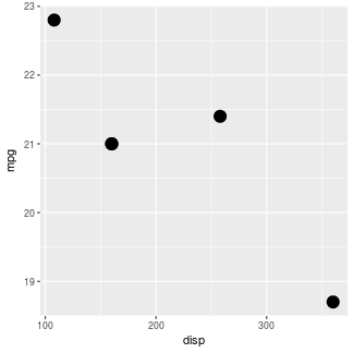
... and calling VI from the 'BrailleR' packge
on the object produces a text description
of the plot ...
VI(g)
  This is an untitled chart with no subtitle or caption.
  It has x-axis 'disp' with labels 100, 200 and 300.
  It has y-axis 'mpg' with labels 19, 20, 21, 22 and 23.
  The chart is a set of 5 points.
  The points are at:
  (160, 21),
  (160, 21),
  (108, 22.8),
  (258, 21.4) and
  (360, 18.7)
  The chart has size set to 5.
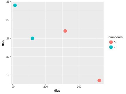
When a plot includes a colour scale, part of the text that
VI generates is a description of the colours used
in the scale. The example below shows this for the same scatterplot,
but with points from different groups drawn with different colours.
g <- ggplot(mtsmall) +
geom_point(aes(x=disp, y=mpg, colour=numgears), size=5)
g
VI(g)
  This is an untitled chart with no subtitle or caption.
  It has x-axis 'disp' with labels 100, 200 and 300.
  It has y-axis 'mpg' with labels 19, 20, 21, 22 and 23.
  There is a legend indicating that colour is used to represent numgears, with 2 levels:
  3 represented by colour #F8766D and
  4 represented by colour #00BFC4.
  The chart is a set of 5 points.
  The points are at:
  (160, 21) colour #00BFC4 which maps to numgears = 4,
  (160, 21) colour #00BFC4 which maps to numgears = 4,
  (108, 22.8) colour #00BFC4 which maps to numgears = 4,
  (258, 21.4) colour #F8766D which maps to numgears = 3 and
  (360, 18.7) colour #F8766D which maps to numgears = 3
  The chart has size set to 5.
For this report, the important part of the above output is the statements about the colour scale, which include a description of the colour of each data point. One of these statements is reproduced below.
[1] "(160, 21) colour #00BFC4 which maps to numgears = 4, "
The problem with this statement is that the colour description,
#00BFC4, is not very meaningful to a human. It is very
difficult to interpret what sort of colour that represents.
The purpose of the 'roloc' package is to provide a framework for converting
this sort of colour description into a more understandable colour
name. For example, the following code shows the result
of calling the colourName function from the 'roloc'
package on this colour
description.
library(roloc)
colourName("#00BFC4")
[1] "turquoise3"
This conversion would allow 'BrailleR' to make statements of the form:
[1] "(160, 21) colour turquoise3 which maps to numgears = 4, "
The conversion from colour specification to colour name involves several different issues:
The following sections deal with each of these issues in turn.
When producing a plot in R, it is possible to specify colours
in several ways. For example, if we wish to draw a plot with
blue data symbols, we can specify the colour using the colour name
"blue", as shown below.
library(ggplot2)
ggplot(mtcars) +
geom_point(aes(x=disp, y=mpg), col="blue")
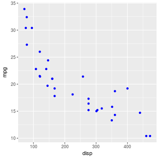
Another way to specify colours is to use a simple numeric index.
R maintains a default colour "palette" and a numeric colour specification
provides an index into that palette. For example, the
default palette is shown below, with "blue" fourth.
palette()
[1] "black" "red" "green3" "blue" "cyan" "magenta" "yellow" "gray"
The following code produces the previous plot by specifying the colour of data points as colour number 4.
ggplot(mtcars) +
geom_point(aes(x=disp, y=mpg), col=4)
Alternatively, we can specify the colour as an RGB triplet, with
two hexadecimal digits for each of red, green, and blue components
(preceded by a hash character).
For example, the code below produces exactly the same blue data
symbols as before, but instead of "blue", we use
"#0000FF" (zero red, zero, green, maximal blue).
ggplot(mtcars) +
geom_point(aes(x=disp, y=mpg), col="#0000FF")
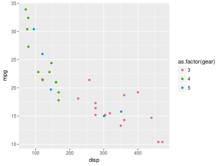
A more complex scenario arises when we want to generate more than
one colour, e.g., to distinguish between different groups on the
same plot. In this case, rather than specifying explicit colours,
we can use a function like hcl to generate a set of
colours. This allows us to obtain results where, for example,
the set of colours differs only in terms of hue, but have
(approximately) equal colourfulness and lightness. The code below
generates red, green, and blue colours that only differ in terms
of hue.
cols <- hcl(c(0, 120, 240), 80, 60)
cols
[1] "#E16A86" "#50A315" "#009ADE"
The following code produces a plot that uses these three colours.
ggplot(mtcars) +
geom_point(aes(x=disp, y=mpg, colour=as.factor(gear))) +
scale_colour_manual(values=cols)
In summary, a colour converter needs to be able to cope with
colours specified by name, by number, or by hexadecimal string.
The following code shows that the colourName function
will accept all three forms of colour specification.
colourName("blue")
[1] "blue"
colourName(4)
[1] "blue"
colourName("#0000FF")
[1] "blue"
Converting a colour specification to a colour name requires two things: a list of colour names to choose from and a way to calculate a match between a colour specification and a colour name.
As a very simple example, we could have the following list of colour names: "red", which corresponds to #FF0000; "green", corresponding to #00FF00; and "blue", #0000FF. If we are given a colour specification, one possibility is that we get a colour specification that is an exact match to our list of colour names. For example, if we are given the colour specification #FF0000, we return the colour name "red". Alternatively, we could get a colour specification that does not match any of the colours in our list. For example, if we are given the colour specification #F0F8FF, what colour name should we return ?
In this section, we will only consider exact matches and we will look at some examples of longer lists of colour names. The Matching colour specifications Section will look at non-exact matches.
There are several possible sources for longer lists of colour names
(and their specifications). For example,
R recognises a list of 657 colour names, whose names are
available via the function colours.
head(colours())
[1] "white" "aliceblue" "antiquewhite" "antiquewhite1" "antiquewhite2" "antiquewhite3"
This is the default list of colour names that is used
by the colourName function. The following code
shows that the colour specification #F0F8FF corresponds to the
colour name "aliceblue" on this list.
colourName("#F0F8FF")
[1] "aliceblue"
That list of colour names is based on a semi-standard set of
"X11" colour names (Jaffer, 2018),
which is very similar to what is used in SVG (Dahlström et al., 2011)
and CSS3 (Tantek et al., 2017).
A much smaller standard set of colour names is the
"HTML" colour names (Bos et al., 2011),
which only contains 16 names.
This set can be used by specifying the colourList
argument to the colourName function.
The code below shows that, for the same colour specification,
different colour lists will sometimes give different colour names.
colourName("#00FF00")
[1] "green"
colourName("#00FF00", colourList=HTMLcolours)
[1] "lime"
It is also possible to create a new list of colour names
with the colourList function. This function
takes two arguments: a character vector of colour names;
and an "sRGB" colour object as produced by
functions in the 'colorspace' package
(Ihaka et al., 2016,
Zeileis et al., 2009), with one sRGB colour
specification per colour name.
The following code
provides a simple example, where the colour list is a set of
colour names that correspond to colours that only differ in terms
of lightness. In this example, the colours are first created
in the CIE LUV colour space (Wikipedia, 2018a)
with the polarLUV function,
so that we can easily control lightness,
then converted to sRGB colours (Wikipedia, 2018b).
library(colorspace)
shades <- colourList(c("light", "medium", "dark"),
                 as(polarLUV(c(100, 50, 0), 0, 0), "sRGB"))
shades
  $names
  [1] "light"  "medium" "dark"

  $colours
               R         G         B
  [1,] 1.0000036 0.9999959 1.0000355
  [2,] 0.4663284 0.4663246 0.4663441
  [3,] 0.0000000 0.0000000 0.0000000

  attr(,"class")
  [1] "colourList"
The colour returned from this colour list can only ever be a shade: either
"light", "medium", or "dark". The following code shows what
happens if we use this colour list with the colourName
function (this also demonstrates that
colourName can convert multiple
colour specifications at once).
colourName(c("#00FF00", "#00BFC4", "#F0F8FF"), colourList=shades)
[1] "light" "medium" "light"
If we have a colour specification that does not exactly match
a colour name in our colour list, we return the closest colour match.
This is what happened in the last example from the previous section;
the colourName function returned the closest shade
name for each colour specification.
In order to decide a closest colour we need to define a colour metric;
a function that can be used to calculate the distance between two
colours. The default colour metric measures euclidean distance in the CIE
LUV colour space, but we can select a different metric via the
colourMetric argument to colourName.
For example, the
euclideanRGB metric measures euclidean distance between
colours within the sRGB colour space. If we use this colour metric,
instead of the default euclideanLUV (keeping
the list of colour names constant),
we will sometimes get
a different result from the same colour specification.
colourName("#F12300")
[1] "firebrick1"
colourName("#F12300", colourMetric=euclideanRGB)
[1] "orangered2"
We can also provide our own function as the
colourMetric argument to the colourName
function. This function must take two
arguments, both of which are "sRGB" objects:
colour is the colour specification that we want to find
a match for and colourList is the list of colours
that we are matching to.
The function must return a matrix of distances with one row
for each colour specification and one column for each
colour in the colour list.
The function may return NA, which means the colour
could not be represented in the colour space used by the colour metric,
and the function may return Inf, which means that
no match could be found for the colour. The latter will
result in the special colour name "unknown".
The code below shows an example of a custom colour metric. This metric works in the CIE LUV colour space, but only considers the lightness component of the colours when determining a match.
lightnessDistance <- function(colour, colourList) {
abs(colour["L"] - colourList[, "L"])
}

lightnessLUV <- function(colour, colourList, ...) {
## Convert 'colour' to 'Luv'
specColour <- as(colour, "LUV")
## Convert 'colourList' to 'Luv'
listColour <- as(colourList, "LUV")
## Calculate distances
specCoords <- coords(specColour)
listCoords <- coords(listColour)
t(apply(specCoords, 1, lightnessDistance, listCoords))
}
The following code uses this colour metric in conjunction with the custom colour list from the previous section to match colours purely on the basis of their lightness.
colourName(c("#00FF00", "#00BFC4", "#F0F8FF"),
       colourList=shades, colourMetric=lightnessLUV)
[1] "light" "medium" "light"
Any additional arguments that are supplied to
colourName are passed on to
the colour metric function
(so the metric function should also have an ellipsis argument, as
demonstrated above).
For example, the default
euclideanLUV colour metric accepts a tolerance
argument. If the distance between a colour specification and
the nearest colour name on the colour list is greater than the
tolerance then the distance Inf is returned for that
comparison. In
the code below, we first return nearest matches, then we specify
a tolerance of zero so that
only exact colour matches are returned (based on the
HTML colour list).
colourName(c("#00FF00", "#00BFC4", "#F0F8FF"),
       colourList=HTMLcolours)
[1] "lime" "aqua" "white"
colourName(c("#00FF00", "#00BFC4", "#F0F8FF"),
       colourList=HTMLcolours, tolerance=0)
[1] "lime" "unknown" "unknown"
There is also a colourNames function, which can return
more than one name for each colour (ordered by increasing distance).
Using the euclideanLUV metric and infinite tolerance,
this will return all colours in the colour list for each
colour match (ordered by increasing distance) ...
colourNames(c("#00FF00", "#00BFC4", "#F0F8FF"),
        colourList=HTMLcolours)
  [[1]]
   [1] "lime"    "green"   "yellow"  "olive"   "aqua"    "teal"    "silver"  "white"   "gray"
  [10] "black"   "navy"    "maroon"  "purple"  "blue"    "red"     "fuschia"

  [[2]]
   [1] "aqua"    "teal"    "silver"  "gray"    "white"   "green"   "navy"    "black"   "olive"
  [10] "purple"  "lime"    "blue"    "yellow"  "maroon"  "fuschia" "red"

  [[3]]
   [1] "white"   "silver"  "gray"    "teal"    "aqua"    "olive"   "green"   "purple"  "navy"
  [10] "black"   "yellow"  "maroon"  "lime"    "blue"    "fuschia" "red"
... or a lower tolerance can be specified to get just "nearby" colours ...
colourNames(c("#00FF00", "#00BFC4", "#F0F8FF"),
        colourList=HTMLcolours, tolerance=40)
  [[1]]
  [1] "lime"

  [[2]]
  [1] "aqua" "teal"

  [[3]]
  [1] "white"  "silver"
The 'roloc' package also
provides a colourSwatch function, which
produces a visual representation of a colour conversion.
This consists of the colour specification
to be matched, and a small rectangle of that colour,
alongside the matched colour name, and a small rectangle of that colour.
This provides some visual feedback on how closely the colour
specification matches the colour name.
colourSwatch(c("#00FF00", "#00BFC4", "#F0F8FF"))

colourSwatch(c("#00FF00", "#00BFC4", "#F0F8FF"),
       colourList=HTMLcolours)

colourSwatch(c("#00FF00", "#00BFC4", "#F0F8FF"),
       colourList=shades, colourMetric=lightnessLUV)

The colourSwatches function is similar,
but it can show more than one match per colour specification.
colourSwatches(c("#00FF00", "#00BFC4", "#F0F8FF"),
           tolerance=5)

colourSwatches(c("#00FF00", "#00BFC4", "#F0F8FF"),
           colourList=HTMLcolours, tolerance=40)

Underlying both of the colourName and
colourSwatch functions is a
lower-level function called colourMatch. This generates
a "colourMatch" object, which contains all of the information
about the comparison of colour specifications with the colour list
and may provide a basis for further calculations on the colour comparison
or for other visualisations of the comparison.
colourMatch(c("#00FF00", "#00BFC4", "#F0F8FF"),
        colourList=shades, colourMetric=lightnessLUV)
  $colour
  [1] "#00FF00" "#00BFC4" "#F0F8FF"

  $colourList
  $names
  [1] "light"  "medium" "dark"

  $colours
               R         G         B
  [1,] 1.0000036 0.9999959 1.0000355
  [2,] 0.4663284 0.4663246 0.4663441
  [3,] 0.0000000 0.0000000 0.0000000

  attr(,"class")
  [1] "colourList"

  $colourDist
            [,1]     [,2]     [,3]
  [1,] 12.264935 37.73508 87.73510
  [2,] 29.653967 20.34605 70.34607
  [3,]  2.821398 47.17862 97.17864

  attr(,"class")
  [1] "colourMatch"
The initial motivation for developing 'roloc' was to provide a tool for the 'BrailleR' package to translate inscrutable colour specifications into more recognisable colour names. However, there are other possible uses of the 'roloc' functionality. For example, any user who encounters a hexadecimal colour specification may find it useful to interactively query a colour specification, as shown below.
colourName("#F8766D")
[1] "salmon"
colourSwatch("#F8766D")

Another possibility is that some colour names themselves are
inscrutable (e.g., "aliceblue" or "lemonchiffon"). Use of
a different (simpler) colour list might provide a translation
of these more exotic names into more familiar terminology.
For example, 'roloc' contains
a simpleColours list with
descriptive labels spread evenly throughout CIE Luv space.
colourName(c("aliceblue", "lemonchiffon"), colourList=simpleColours)
[1] "greyish very light blue" "dull very light yellow"
colourSwatch(c("aliceblue", "lemonchiffon"), colourList=simpleColours)

The 'roloc' package makes it easy to add further colour lists and colour metrics. For example, it should be easy to create a colour list based on the XKCD colour survey Munroe, 2010.
One possible use of this flexibility is to provide non-english
colour lists.
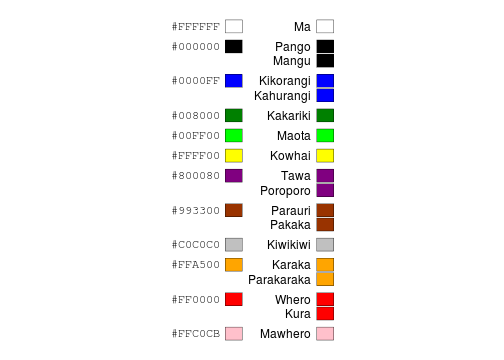
For example, the 'roloc' package contains a
NgaTae colour list with some basic Maori colour names.
colourSwatches(rgb(unique(coords(NgaTae$colours))), colourList=NgaTae, tolerance=0)
A discussion on the R-help mailing list from 2013
about "measuring distances between colours?" includes a function
rgb2col by Kevin Wright, which works very much like the
default settings for the colourName function (it matches
R colour names using euclidean distance in CIE LUV space).
The 'roloc' package was developed in (shameful) ignorance of this
discussion, but provides greater flexibility by allowing
different colour lists and different colour metrics to be specified.
There are many R packages that deal with colour, but none were found that deal directly with the problem of converting colour specifications to colour names. Numerous packages provide functions for generating colour palettes, for example, 'RColorBrewer' (Neuwirth, 2014) and 'pals' (Wright, 2017), and the 'colorscience' package (Gama, 2017) contains a large number of colour resources including colour space conversions, and colour metrics. The 'roloc' package builds on the 'colorspace' package for representing colour specifications in different colour spaces and transforming between colour spaces.
Outside of R, there are a number of web sites that provide conversions from colour specifications to colour names, for example, http://shallowsky.com/colormatch/index.php, which includes links to its PHP source code. There are also standalone programs like The Known Colors Palette Tool and there are numerous mobile phone apps, such as Color Grab (Loomatix), ColourMatch (Resene), and Color ID (GreenGar). However, all of these lack the flexibility and/or programmability of a general software package and, of course, cannot be easily used from R.
The 'roloc' package provides tools for converting colour specifications
to colour names. The main function is colourName, which
accepts any R colour specification and returns a character vector
of colour names. The user can
select a list of colour names to match against
and a metric function to determine the closest colour.
The examples and discussion in this document relate to version 0.1 of the 'roloc' package and version 0.27 of the BrailleR package.
This report was generated within a Docker container (see Resources section below).
Murrell, P. (2018). "Generating Colour Names: The 'roloc' Package for R." Technical Report 2018-01, Department of Statistics, The University of Auckland. [ bib ]

This document
by Paul
Murrell is licensed under a Creative
Commons Attribution 4.0 International License.