'gggrid' it's g-g-great!

Accessing 'grid' from 'ggplot2'

Paul Murrell
The University of Auckland
2021

Title slide.

Suppose we want to create a plot like this

Let us suspend disbelief for a moment and suppose that this is actually a plot someone would want to create.

A plot with a radial gradient fill on top of the data

"This" being a 'ggplot2' plot with a radial gradient fill drawn on top.

Good News

library(grid)
grad <- radialGradient(c(rgb(0,0,0,0), "black"))
grid.rect(gp=gpar(fill=grad))

'grid' can draw radial gradients (from R 4.1.0) NOTE the rgb(0,0,0,0) instead of "transparent" because "transparent" in R is transparent *white* !

More Good News

'ggplot2' is built on top of 'grid'

Bad News

'ggplot2' is ashamed of 'grid'

library(ggplot2)
viewport()

Error in viewport(): could not find function "viewport"

'ggplot2' provides a higher-level interface with its own concepts of geoms and aesthetics etc. 'ggplot2' does not expose 'grid' concepts like viewports and units.

More Bad News

?ggplot2::colour

     Colours and fills can be specified in the following ways:

         A name, e.g., ‘"red"’. R has 657 built-in named colours,
          which can be listed with ‘grDevices::colors()’.

         An rgb specification, with a string of the form ‘"#RRGGBB"’
          where each of the pairs ‘RR’, ‘GG’, ‘BB’ consists of two
          hexadecimal digits giving a value in the range ‘00’ to ‘FF’.
          You can optionally make the colour transparent by using the
          form ‘"#RRGGBBAA"’.

         An ‘NA’, for a completely transparent colour.

'ggplot2' does not (yet) provide a higher-level interface to radial gradients. And every time something new is added to 'grid' you have to wait for someone to add a 'ggplot2' interface to give you access.

ggplot(mtcars, aes(disp, mpg)) + geom_point()
library(grid)
grid.force()
downViewport("panel.7-5-7-5")
grid.rect(gp=gpar(fill=grad))

It *is* possible to combine 'grid' with 'ggplot2', but there are some drawbacks: grid.force() is a bit mysterious. "panel.7-5-7-5" is a bit mysterious. You need to know quite a bit about both 'ggplot2' and 'grid' to do this. This is not easy to teach! AND you are just drawing on top of everything.

downViewport("panel.7-5-7-5")
current.viewport()$xscale

[1] 0 1

AND you DO NOT have access to the coordinate system on the 'ggplot2' axes. So this is at best a mixture of good news and bad news.

library(gggrid)
ggplot(mtcars, aes(disp, mpg)) +
    geom_point() +
    grid_panel(rectGrob(gp=gpar(fill=grad)))

Isn't that a whole lot nicer ? You just add a 'grid' grob to your 'ggplot2' plot.

grid.rect(gp=gpar(fill=grad))

r <- rectGrob(gp=gpar(fill=grad))
grid.draw(r)

The only thing to learn is the idea of a "grob". That is a lot easier to teach.

library(gggrid)
ggplot(mtcars, aes(disp, mpg)) +
    grid_panel(rectGrob(gp=gpar(fill=grad))) +
    geom_point(color="white")

You can even add the 'grid' grob ahead of other 'ggplot2' layers if you like.

gradFun <- function(data, coords) {
    rectGrob(gp=gpar(fill=grad))
}
ggplot(mtcars, aes(disp, mpg)) +
    geom_point() +
    grid_panel(gradFun)

The argument to grid_panel() can be a function.

debugData <- function(data, coords) {
    print(head(data))
}

ggplot(mtcars, aes(x=disp, y=mpg)) +
    geom_point() +
    grid_panel(debug=debugData)

    x    y PANEL group
1 160 21.0     1    -1
2 160 21.0     1    -1
3 108 22.8     1    -1
4 258 21.4     1    -1
5 360 18.7     1    -1
6 225 18.1     1    -1

The panel function gets called with the data for each panel. This effectively gives us access to the plot scales. We can see the raw data for the panel.

debugCoords <- function(data, coords) {
    print(head(coords))
}

ggplot(mtcars, aes(x=disp, y=mpg)) +
    geom_point() +
    grid_panel(debug=debugCoords)

          x         y PANEL group
1 0.2470464 0.4555126     1    -1
2 0.2470464 0.4555126     1    -1
3 0.1291299 0.5251451     1    -1
4 0.4692737 0.4709865     1    -1
5 0.7005714 0.3665377     1    -1
6 0.3944421 0.3433269     1    -1

And we can see the transformed data for the panel.

The function gets called for each panel so we can draw 'grid' output in different panels. We can use the data for each panel to draw something DIFFERENT on each panel.

Output from previous slide.

gradFun <- function(data, coords) {
    grad <- radialGradient(c("transparent",
                             adjustcolor(data$colour[1], alpha=.5),
                             "transparent"))
    cx <- mean(coords$x)
    cy <- mean(coords$y)
    rectGrob(cx, cy, gp=gpar(col=NA, fill=grad))
}

ggplot(mtcars, aes(disp, mpg, colour=factor(am))) +
    geom_point() +
    grid_group(gradFun)

There is also a grid_group() function. That function gets called with the data for each group. The argument to grid_group() can be a grob (draw the same thing for each group) or a function, so we can draw 'grid' output for different groups.

Output from previous slide.

Summary

'ggrid' makes it easy to add a 'grid' grob (or function) to a 'ggplot2' plot.
We also get to draw the grob (or function) before or after other 'ggplot2' drawing.
We also get access to the 'ggplot2' coordinate system for locating our 'grid' drawing.

Summary slide.

GALLERY

A set of examples of 'gggrid' in use.

bgrect <- function(data, coords) {
    rectGrob(gp=gpar(col=NA, fill=adjustcolor(data$fill[1], alpha=.3)))
}
ggplot(df, aes(x=date, y=vari)) +
    grid_panel(bgrect, aes(fill=geo)) +
    scale_fill_manual(values=colr) +
    geom_bar(stat="identity") + facet_grid(est ~ geo)

The interesting thing here is the use of aes(fill=geo) and scale_fill_manual() that make use of the 'ggplot2' infrastructure to select and map colours to data values, then drawing 'grid' shapes with those colours (to create a background for each panel). It also demonstrates the usefulness of accessing raw 'grid' - there is a ggplot2::geom_rect(), but to get it to fill the plot region you have to use the awkward 'xmin = -Inf'. A rectGrob() has access to 'grid' coordinates like "npc", where "left" is just 0 and "right" is just 1.

ggplot(data = mtcars,
       mapping = aes(x    = mpg,
                     y    = wt,
                     size = cyl,
                     fill = as.factor(cyl))) +
    gggrid::grid_panel(panel_func) +
    theme_bw()

The interesting bit here is using the aesthetics from the 'ggplot2' mappings to control the colour and size (and x/y location) of the custom data symbols. The usefulness of 'gggrid' here is that we can draw a data symbol that 'ggplot2' does not already have. This comes from the "coolbutuseless" blog. Try not to read too much into the name ...

Turns out, at least one person does want to draw a radial gradient on top of a 'ggplot2' plot!!! The usefulness of 'gggrid' here is that 'ggplot2' does not provide an interface to radial gradients, so we need access to raw 'grid'.

Acknowledgements

Philip Smith

https://stat.ethz.ch/pipermail/r-help/2021-October/472658.html

Mike FC

https://coolbutuseless.github.io/2021/11/04/custom-ggplot2-point-shapes-with-gggrid/

David Stomski

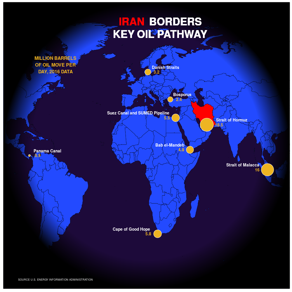
https://www.stomperusa.com/2020/02/08/replicating-plots-oil-pathways/
https://www.stomperusa.com/2021/10/06/replicating-plots-oil-pathways-with-radial-gradient/

Acknowledgements for Gallery examples.

References

Murrell, P. (2021). "Accessing 'grid' from 'ggplot2'" Technical Report 2021-01, Department of Statistics, The University of Auckland. version 1.

https://stattech.wordpress.fos.auckland.ac.nz/2021/05/31/2021-01-accessing-grid-from-ggplot2/

Murrell, P. (2021). gggrid: Draw with 'grid' in 'ggplot2'. R package version 0.1-1.

https://github.com/pmur002/gggrid

Links to tech report and software.