Making Colour Accessible

Paul Murrell
The University of Auckland
March 2018

This talk will describe some recent work that I have done on accessibile statistical graphics and colour. I am going to emphasise the journey rather than just the destination, reflect upon some of the joys of working in the field of Statistical Computing and Graphics, and attempt to drawing out some general wisdom about creating software, which is mostly what I do. It is customary to begin a talk with an outline of the talk; a sort of table of contents. But I am not going to do that because it would give away the ending. You will just have to stay awake all the way through.

BrailleR

A histogram

library(BrailleR)
p <- hist(faithful$eruptions)

The hist() function can draw a histogram AND it returns information about the histogram that it drew.

BrailleR

'BrailleR' package can generate text from plots

VI(p)

This is a histogram, titled: Histogram of faithful$eruptions
"faithful$eruptions" is marked on the x-axis.
Tick marks for the x-axis are at: 2, 3, 4, and 5 
There are a total of 272 elements for this variable.
Tick marks for the y-axis are at: 0, 20, 40, and 60 
It has 8 equal-width bins, starting at 1.5 and ending at 5.5 .
The mids and counts for the bins are:
mid = 1.75  count = 55 
mid = 2.25  count = 37 
mid = 2.75  count = 5 
mid = 3.25  count = 9 
mid = 3.75  count = 34 
mid = 4.25  count = 75 
mid = 4.75  count = 54 
mid = 5.25  count = 3

The VI() function from the 'BrailleR' package takes the information about a histogram and turns it into a text description of the histogram. In combination with a screen reader, this provides some information about the histogram for blind or visually impaired R users.

ggplot2

A 'ggplot2' plot

library(ggplot2)
g <- ggplot(faithful) +
 geom_histogram(aes(x=eruptions), breaks=p$breaks)

The 'ggplot2' package is a very popular package for generating plots in R

ggplot2 in BrailleR

Debra Warren added support for ggplot2 to BrailleR

VI(g)

This is an untitled chart with no subtitle or caption.
It has x-axis 'eruptions' with labels 2, 3, 4 and 5.
It has y-axis 'count' with labels 0, 20, 40 and 60.
The chart is a bar chart containing 8 vertical bars.
Bar 1 is centered at 1.75, and spans vertically from 0 to 55.
Bar 2 is centered at 2.25, and spans vertically from 0 to 37.
Bar 3 is centered at 2.75, and spans vertically from 0 to 5.
Bar 4 is centered at 3.25, and spans vertically from 0 to 9.
Bar 5 is centered at 3.75, and spans vertically from 0 to 34.
Bar 6 is centered at 4.25, and spans vertically from 0 to 75.
Bar 7 is centered at 4.75, and spans vertically from 0 to 54.
Bar 8 is centered at 5.25, and spans vertically from 0 to 3.

Debra Warren, in a Masters Project, added support for 'ggplot2' plots in 'BrailleR'

ggplot2 in BrailleR

A 'ggplot2' plot with colour

gCol <- ggplot(faithful) +
    geom_histogram(aes(x=eruptions, fill=eruptions > 3),
                   breaks=p$breaks)

The text description generated from a 'ggplot2' plot includes information about colour scales used in the plot.

ggplot2 in BrailleR

One small detail left unsolved by Debra's work was the translation of colour settings in plots

VI(gCol)

This is an untitled chart with no subtitle or caption.
It has x-axis 'eruptions' with labels 2, 3, 4 and 5.
It has y-axis 'count' with labels 0, 20, 40 and 60.
Fill is used to represent eruptions > 3, with 2 levels:
FALSE represented by fill #F8766D and 
TRUE represented by fill #00BFC4.
The chart is a bar chart containing 16 vertical bars.

#RRGGBB colour specifications are hard to understand

The text description of colour reports colours in the #RRGGBB format that R uses for colours, which is not very easy for a human audience to interpret. #RRGGBB gives the amount of red, green, and blue as pairs hexdecimal digits. Each pair ranges from 00 to FF. For example: #F8766D is lots of red and medium amounts of green and blue (and light reddish something or other); #00BFC4 is no red, but quite a lot of both green and blue (some sort of turquoise).

Colour Names

The basic problem is to turn a colour specification into a colour name

library(roloc)
colourName("#FF0000")

[1] "red"

colourSwatch("#FF0000")

The solution to every problem is an R package!

The 'roloc' package was created to convert #RRGGBB colour specifications into colour names. If all we were going to talk about was the ending, that would be it; job done. But the more interesing part is how we got here ...

Colour Names

R has a (quite large) set of colour names

head(colours(), 20)

 [1] "white"         "aliceblue"     "antiquewhite" 
 [4] "antiquewhite1" "antiquewhite2" "antiquewhite3"
 [7] "antiquewhite4" "aquamarine"    "aquamarine1"  
[10] "aquamarine2"   "aquamarine3"   "aquamarine4"  
[13] "azure"         "azure1"        "azure2"       
[16] "azure3"        "azure4"        "beige"        
[19] "bisque"        "bisque1"

length(colours())

[1] 657

One issue that 'roloc' faced was what colour names to use. R contains a long list of colour names. This list is very similar to colour names that we can use in CSS and SVG.

Colour Names

But there are other sets of colour names too

There is also a list of "simple" HTML colours.

Colour Names

And there are other sets of colour names too

https://blog.xkcd.com/2010/05/03/color-survey-results/

XKCD also has a list of colour names based on a large online survey. Put simply, the list of colour names that people use is not completely obvious and there are several ways to do it.

Colour Names

So 'roloc' lets you choose

colourSwatch("#FF0000", colourList=NgaTae)

programming tip #1:
if a decision is difficult, don't make it

Because it was not clear which list of colour names was best (for all purposes), this became a parameter of the 'roloc' functions; the user can select the list of colour names (with the R colours as the default). The general software creation wisdom from this situation is: if you see multiple ways to do something and you cannot see a clear winner, leave your options open.

Colour Metrics

No matter which colour list we choose, there are MANY more colour specifications than colour names

16*16*16*16*16*16

[1] 16777216

2^24

[1] 16777216

A list of colour names has an #RRGGBB colour associated with each name. But there are many #RRGGBB colour specifications with no corresponding colour name.

Colour Metrics

So we need to calculate the "closest" colour name

For a particular #RRGGBB colour specification, we need to find the "closest" colour name, but we need a metric that we can use to measure "distance" between colour specifications.

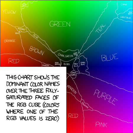
Colour Metrics

RGB is a 3D space

All #RRGGBB colour specifications can be visualised as a 3D cube, with the amount of red on one dimension, the amount of green on another, and blue on the third dimension.

Colour Metrics

so we could just use (RGB) euclidean distance

The distance between #RRGGBB colours can be calculated as just the length of the straight line between the colours in RGB space.

Colour Metrics

But there are other colour spaces

Like CIE XYZ

But there are problems with RGB space. For example, RGB is not perceptually uniform; a distance of 1 in one part of RGB space does not appear the same size as a distance of 1 in another part of RGB space. This means that RGB is not a very good space to perform distance calculations within. There are other colour spaces, like CIE XYZ, and it is possible to convert between these colour spaces.

RGB to XYZ

$$v \in \{r, g, b\}$$ $$V \in \{R, G, B\}$$

$$v = \left\{\begin{array}{l l} V/12.92 & \mathrm{if}\ V \leq 0.04045 \\ ((V + 0.055)/1.055)^{2.4} & \mathrm{otherwise} \end{array}\right.$$

$$\left[ \matrix{X \\ Y \\ Z} \right] = \left[ \matrix{ 0.4124564 & 0.3575761 & 0.1804375 \\ 0.2126729 & 0.7151522 & 0.0721750 \\ 0.0193339 & 0.1191920 & 0.9503041} \right] \left[ \matrix{r \\ g \\ b}\right]$$

All these formulas are designed to show is that there is a mathematical relationship between RGB and XYZ. This means that we can take any RGB colour and calculate an XYZ specification for the colour.

Colour Metrics

And there are other colour spaces

Like CIE Luv (which is more perceptually uniform)

Another colour space is CIE Luv. The value of this colour space is that it is (more) perceptually uniform. This means that it is a better space to perform calculations of distance within.

XYZ to Luv

$$L = \left\{\begin{array}{l l} 116 \sqrt[3]{y_r} - 16 & \mathrm{if}\ y_r > 0.008856 \\ 903.3 y_r & \text{otherwise} \end{array}\right.$$

$$u = 13 L (u' - u_r')$$

$$v = 13 L (v' - v_r')$$

\begin{array}{l l} y_r = {{Y} \over {Y_r}} & v' = {{9Y} \over {X + 15Y + 3Z}} \\ u_r' = {{4X_r} \over {X_r + 15Y_r + 3Z_r}} & v_r' = {{9Y_r} \over {X_r + 15Y_r + 3Z_r}} \end{array}

These formulas are designed just to show that there is a mathematical relationship between XYZ and Luv. So we can take any RGB colour and generate an Luv colour.

Colour Metrics

So 'roloc' lets you choose

colourSwatch("#FF0000", colourMetric=euclideanLUV)

However, there are still more colour spaces and there may be different contexts within which we wish to determine "closeness", so again we allow the user to select how to measure distances between colours. So now we have the ability to choose a colour list and a colour metric to perform the conversion from colour specification to colour name.

Software Design

Note that colourName() and colourSwatch() do the same thing; they just present the results differently

colourName("#FF0000", colourList=NgaTae)

[1] "Whero"

colourSwatch("#FF0000", colourList=NgaTae)

Notice that 'roloc' presents the conversion in two ways: a simple character vector and a colour swatch graphic.

Software Design

So 'roloc' has colourMatch()

colourMatch(c("#FF0000"), colourList=NgaTae)$colourDist

        [,1]     [,2]     [,3]     [,4]     [,5]     [,6]
[1,] 185.045 186.7891 186.7891 250.4087 250.4087 219.7092
         [,7]     [,8]    [,9]   [,10]    [,11]    [,12]
[1,] 269.5398 186.2394 163.493 163.493 95.29694 95.29694
        [,13]    [,14]    [,15] [,16] [,17]    [,18]
[1,] 180.7035 108.7122 108.7122     0     0 144.6701

colourName() and colourSwatch() use colourMatch()

There is actually a function underneath called colourMatch() that does the actual conversion; both colourName() and colourSwatch() use that function to get the result and just present the result in different ways.

Software Design

Also note that it is possible for a single colour spec to match more than one colour name

col2rgb(c("#FF0000", "red", "red1"))

      [,1] [,2] [,3]
red    255  255  255
green    0    0    0
blue     0    0    0

We can also see that some colour names correspond to exactly the same colour specification. Here, both "red" and "red1" correspond to the colour specification "#FF0000".

Software Design

So 'roloc' has colourNames() and colourSwatches()

colourNames("#FF0000", tolerance=0)

[[1]]
[1] "red"  "red1"

colourSwatches("#FF0000", tolerance=0)

Both of these also use colourMatch()

The 'roloc' package has two more functions, colourNames() and colourSwatches(), that allow for multiple colour names matching a colour specification. We have functions that report the closest colour name match AND we have functions that report the "N" closest colour name matches. Both of these functions are also built upon the colourMatch() function.

Software Design

programming tip #2:
if your tummy does not feel all warm inside,
you have not got it right yet

The design of the functions within the 'roloc' package is satisfying because: there is a single function that calculates all of the information needed to determine a matching colour name; there are separate functions for a single match and for multiple matches, because those are different types of results; although both of the "swatch" functions produce the same type of result, there are two different functions to match the two functions that produce character results. The general software wisdom from this situation is: the design of functions within a package often requires thought and refactoring, but it is very satisfying when you get it right. You can tell that you have not got it right yet when it feels awkward and inelegant.

Half-time Interval

We have built a tool to help solve the problem

library(RColorBrewer)
oranges <- brewer.pal(6, "Oranges")

Let's assess how well the default tool settings work with some half-time oranges

This is the half-way point in the story. We have the 'roloc' package and it is elegant and heart-warming. But how well does it solve the original problem ? Here are 6 different shades of orange; how well does 'roloc' do at converting these to colour names?

Colour Names

The colour names are not always clear

colourSwatch(oranges)

The original problem was that I could not easily understand the #RRGGBB colour specifications, but now I have a new problem: I cannot easily understand the colour names! (for some colour lists) What colour does the name "burlywood1" conjure up for you?

Colour Names

And the colour names are not always accurate

colourSwatch(oranges, colourList=NgaTae)

Another problem is that some colour lists are not detailed enough; everything just comes out "Karaka"

Colour Names

But I am not unhappy because my job is to create the right infrastructure

It is not my fault if a colour list is useless

programming tip #3:
build a fishing rod, not a fish

Fortunately, because I designed 'roloc' so well, this is not a disaster. I can blame it all on the limitations of the colour lists. The general software wisdom in this situation is: It is much more fun to create general software tools that solve sets of problems than it is to create specific solutions.

Colour Names

We have built a tool, now let's try using it to solve the problem better

Our task now is to find a colour list and a colour metric that does a better job

On the other hand, it is good to actually produce a useful solution. This is the second half of our story - finding a colour list that produces understandable and accurate colour names.

ISCC-NBS Colour Names

The ISCC-NBS System of Colour Designation offers hope

"A means of designating colors ... sufficiently standardized as to be acceptable and usable by science, sufficiently broad to be appreciated and used by science, art, and industry, and sufficiently commonplace to be understood, at least in a general way, by the whole public."

The definition of the ISCC-NBS System of Colour Designation certainly sounds like it should fit the bill.

ISCC-NBS Colour Names

The ISCC-NBS System of Colour Designation offers hope

The ISCC-NBS system contains understandable colour names that can still discern between quite similar-looking colours.

ISCC-NBS Colour Names

But the ISCC-NBS System of Colour Designation is based on the Munsell colour system

But making use of the ISCC-NBS system is not going to be straightforward. The first obstacle is that ISCC-NBS is defined in terms of the Munsell colour space; this is a very beautiful and well-structured colour space, but it does NOT have a very simple relationship with RGB.

ISCC-NBS Colour Names

And the ISCC-NBS colour names correspond to regions of colour space, not just single locations

Furthermore, ISCC-NBS colour names correspond to regions of Munsell colour space (not single points in colour space). This means that "distance" has to be calculated differently.

ISCC-NBS Colour Names

So we need to get from the RGB colour space to the ISCC-NBS colour system

In order to get an ISCC-NBS colour list for use with 'roloc', we need to be able to convert RGB colour specifications into Munsell colours. Note that this conversion goes via yet another colour space called CIE xyY.

ISCC-NBS Colour Metric

And we need to provide a distance metric based on colour regions.

colourMatch(c("#FF0000"), colourList=NgaTae,
    colourMetric=ISCCNBSblock)$colourDist

     [,1] [,2] [,3] [,4] [,5] [,6] [,7] [,8] [,9] [,10]
[1,]  Inf  Inf  Inf   NA   NA  Inf  Inf   NA  Inf   Inf
     [,11] [,12] [,13] [,14] [,15] [,16] [,17] [,18]
[1,]   Inf   Inf   Inf   Inf   Inf     0     0   Inf

If a colour specification lies within a region, its distance to that region is zero, otherwise its distance is infinity. This is another reason for allowing multiple colour name matches; it is possible for more than one colour name to lie within the same ISCC-NBS colour block (as the colour specification).

ISCC-NBS Colour Names

But converting from RGB to Munsell is hard because there is no general equation

Unfortunately, there is no mathematical equation to transform from RGB to Munsell. We only have a known conversion for a finite set of Munsell colours.

Color-Science.org

But there is a package called 'colorscience' that can convert from sRGB to xyY

library(colorscience)
xyY <- XYZ2xyY(RGB2XYZ(t(col2rgb("#FF0000"))/255,
               illuminant="C"))
xyY

          [,1]      [,2]      [,3]
[1,] 0.6396045 0.3281296 0.2145626

The conversion as far as CIE xyY is pretty easy - it is the next step, from xyY to Munsell that is hard.

Color-Science.org

And there is a Python package called 'colour' that can perform the transformation from xyY to Munsell

And there is a package called 'reticulate' that can call Python code from R

library(reticulate)
colour <- import("colour")
munsell <- colour$xyY_to_munsell_colour(xyY)
munsell

[1] "7.8R 5.2/20.6"

Fortunately, there is a Python package called 'colour' that can perform the conversion from xyY to Munsell. There is also an R package that lets us call Python code from R.

Color-Science.org

And the package called 'colorscience' can also convert from Munsell to ISCC-NBS

ColorBlockFromMunsell(MunsellSpecToHVC(munsell))

[1] "vivid reddish orange"

programming tip #4:
BE LAZY

And the final step from Munsell to ISCC-NBS is also pretty easy. So all we have to do is connect these packages together. The software wisdom from this situation is: make use of existing solutions where possible; it not only saves you time, but code that has been out there and used by lots of other people is going to be much more robust than code you write for yourself.

Package Dependencies

But using the Python package 'colour' requires Python and that is a nuisance (as a package dependency)

programming tip #5:
Not everyone uses Linux

The bad news is that this jigsaw solution does not fit nicely into an R package because the Python part places a large burden on the end user to install Python and the 'colour' package. And that is not straightforward on Windows. The software wisdom from this situation is: for a solution to be useful, it must be portable.

Precalculation

But what if we precalculated the conversions ?

      RGB       name                  
 [1,] "#730A0A" "deep reddish brown"  
 [2,] "#740A0A" "deep reddish brown"  
 [3,] "#750A0A" "deep reddish brown"  
 [4,] "#760A0A" "deep reddish brown"  
 [5,] "#770A0A" "deep reddish brown"  
 [6,] "#780A0A" "deep reddish brown"  
 [7,] "#790A0A" "strong reddish brown"
 [8,] "#7A0A0A" "strong reddish brown"
 [9,] "#7B0A0A" "strong reddish brown"
[10,] "#7C0A0A" "strong reddish brown"
[11,] "#7D0A0A" "strong reddish brown"

One way around this problem is to use the Python package to do all possible conversions and just include the pre-calculated conversions with the package.

Precalculation

There are LOTS of sRGB specifications, but the number is finite

16*16*16*16*16*16

[1] 16777216

2^24

[1] 16777216

This is a lot of conversions, but it is a finite number.

Slow Code

But it takes quite a while to do LOTS of calls to xyY_to_munsell_colour()

Unfortunately it takes a long time to run all of the xyY to Munsell conversions ...

Slow Code

But it takes quite a while to do LOTS of calls to xyY_to_munsell_colour()

## Seconds
round(2^24/1000*4)

[1] 67109

## Minutes
round(2^24/1000*4/60)

[1] 1118

## Hours
round(2^24/1000*4/60/60)

[1] 19

... pretty much an entire day in fact.

Parallel code

But the calculations are embarassingly parallel

programming tip #6:
Computers can multitask

Fortunately, each conversion is independent of every other conversion, so we can run them in parallel and bring the time down considerably. The software lesson from this situation is: modern computers have multiple CPUs and it is very useful to know how to get all of them working at once. This is pretty easy to do in R.

Slow R Code

But it takes even longer to do LOTS of calls to ColorBlockFromMunsell()

Unfortunately, the Munsell to ISCC-NBS conversion is even slower. The important feature of this graph is that it is exponential; it gets steeper and steeper.

Slow R Code

Because ColorBlockFromMunsell() is not very efficient

ColorBlockFromMunsell <- function(HVC) {
    ...
    out = data.frame(HVC=HVC, Number=as.integer(NA),
           Name=as.character(NA),
           stringsAsFactors=FALSE )
    for (i in 1:nrow(out)) {
        result  = ColorBlockFromMunsell( HVC[i, ] )
        out$Number[i]   = result$Number
        out$Name[i]     = result$Name
    }
    ...
}

The reason it is slow is because it has a loop that incrementally grows an R data frame (so there is a LOT of copying of objects in memory).

Refactoring Code

But a vectorised version of ColorBlockFromMunsell() is MUCH faster

We can write a vectorised (non-loop) version of the ColorBlockFromMunsell() function and that makes it MUCH faster. The shallow straight line is the new, faster version.

Sharing Code Fixes

And a vectorised version of ColorBlockFromMunsell() is possible because 'colorscience' is Open Source

This sort of fix is possible because R packages tend to be open source, so we can see the code, copy the code, modify the code ...

Sharing Code Fixes

And a vectorised version of ColorBlockFromMunsell() can give back and be tracked through version control

programming tip #7:
Sharing makes your tummy all warm inside

... and share our new code. Using version control systems like github allows those changes to be tracked against the original code and supports ongoing copying, modification, and sharing with others. The software wisdom from this situation is: an open source community generates an environment where sharing is the norm. This leads to better communication and resolution of problems. It also leads to a friendly, supportive, and generous environment that is very pleasant to work in.

Storage

But the result is VERY large (too large for a package)

print(object.size(expand.grid(0:255, 0:255, 0:255)),
      units="Mb")

192 Mb

Unfortunately, the final set of RGB colour specifications plus ISCC-NBS colour names is very large - way too large to distribute as an R package.

Storage

But we can be be clever/sneaky

But we do not actually need to store all of the RGB specifications; we can just remember the order in which we generated the specifications (and the colour names).

Storage

But we can be be clever/sneaky

file.size(system.file("extdata", "block.rds",
              package="rolocISCCNBS"))

[1] 2820663

2.7 MB is small enough for an R package.

If we do this, and if we store the colour names as an R object (rather than a text file), then we only really store every unique colour name, and the size of the pre-calculated colour name object comes WAY down.

Colour Names

Are we doing better?

library(rolocISCCNBS)
colourSwatch(oranges, colourList=ISCCNBScolours,
     colourMetric=ISCCNBSblock)

So we now have another R package, 'rolocISCCNBS', which contains an ISCC-NBS colour list and an ISCC-NBS colour metric. How does it do on the set of orange colour specifications? Not bad (?)

Summary

Started with a small problem
Made a tool to help solve the problem
Learned a lot about colour
Took other people's code
Gave back fixes for other people's code
Encountered computational problems
Applied HPC and cleverness
It is not clear how useful the end result will be,
but the journey was awesome and
it was satisfying to solve the problem properly

So this is the somewhat disappointing ending. We may have created a colour specification to colour name conversion that performs reasonable well and this will provide a little bit of help to a small community of R users with accessibility issues. But it was a lot of fun getting to this point. And it was still very rewarding to produce a solution that is elegant, flexible, and extensible.

Acknowledgements

'BrailleR' is the brain child of Jonathon Godfrey
The 'ggplot2' support in 'BrailleR' was developed by Debra Warren

Final Word

This work owes several debts of gratitude to
Ross Ihaka:

The success of R has created breathing space for people to work on problems and solutions that may not have an immediate impact
The early work on R demonstrates the value of making good tools for others to build on
The openness of R has lead to a Statistics community where sharing is the norm