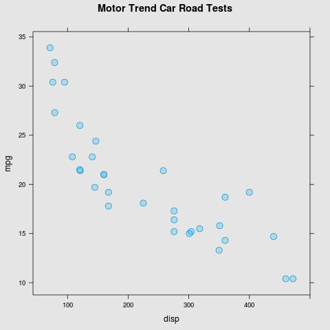
PNG Graphics ============<img src="plot.png"/>Pros : * You can produce **any** R plot Cons : * The graphic is **static** * Raster graphics **do not scale** SVG Graphics ============ ```{r results="hide"} svg("plot.svg") print(latticePlot) dev.off() ``` ```{r echo=FALSE, results="hide"} svg("plot.svg", width=7, height=7) print(latticePlot) dev.off() ```

SVG Graphics ============<img src="plot.svg"/>Pros : * You can produce **any** R plot * Vector graphics **scale** Cons : * The graphic is **static** * You are **limited to R graphics concepts** gridSVG Graphics ================ ```{r results="hide", message=FALSE} library(gridSVG) ``` ```{r results="hide"} gridsvg("gridsvg-plot.svg", prefix="gridsvg-") print(latticePlot) dev.off() ``` gridSVG Graphics ================
<img src="gridsvg-plot.svg"/>Cons : * You can only produce **graphics based on grid** Pros : * Vector graphics **scale** * You have access to **SVG concepts** R Graphics ========== ```{r eval=FALSE, echo=FALSE, results="hide", warning=FALSE, message=FALSE} # No longer used svg("r-graphics.svg") library(gridGraphviz) nodes <- c("ggplot2", "lattice", "grid", "graphics", "grDevices", "gridSVG", "PNG", "SVG") gnel <- new("graphNEL", nodes=nodes, edgeL=list(ggplot2=list(edges="grid"), lattice=list(edges="grid"), grid=list(edges=c("grDevices", "gridSVG")), graphics=list(edges="grDevices"), grDevices=list(edges=c("PNG", "SVG")), gridSVG=list(edges="SVG"), PNG=list(), SVG=list()), edgemode="directed") shapes <- rep(c("circle", "box"), c(6, 2)) names(shapes) <- nodes colours <- rep(c("black", "white"), c(6, 2)) names(colours) <- nodes fills <- rep(c("grey", "black"), c(6, 2)) names(fills) <- nodes arrows <- rep("normal", 8) names(arrows) <- edgeNames(gnel) rag <- agopen(gnel, "", attrs=list(graph=list(fixedsize="false")), nodeAttrs=list(shape=shapes, fontcolor=colours, fillcolor=fills), edgeAttrs=list(arrowhead=arrows)) grid.newpage() grid.graph(rag) dev.off() ```

gridSVG: Only grid-based output ================ ```{r results="hide"} png("graphics.png") plot(mpg ~ disp, mtcars) dev.off() ``` ```{r echo=FALSE, results="hide"} png("graphics.png") plot(mpg ~ disp, mtcars, pch=16) grid.rect(gp=gpar(fill=NA)) dev.off() ```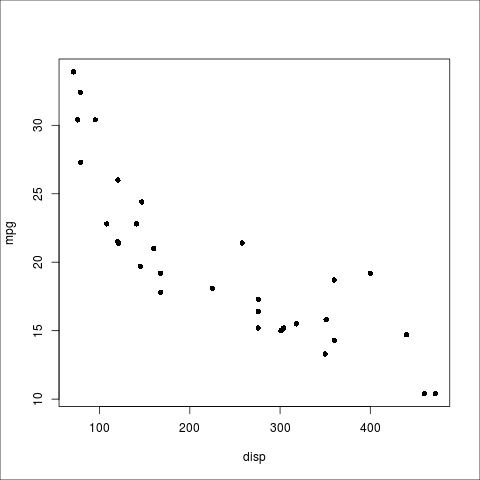
gridSVG: Only grid-based output ================ ```{r results="hide", warning=FALSE} gridsvg("graphics.svg") plot(mpg ~ disp, mtcars) dev.off() ``` ```{r echo=FALSE, results="hide"} gridsvg("base.svg", prefix="base-") grid.rect() plot(mpg ~ disp, mtcars) dev.off() ``` gridSVG: The grid Display List ======= ```{r results="hide"} gridsvg("gridsvg-plot.svg", prefix="gridsvg-") print(latticePlot) dev.off() ``` gridSVG: The grid Display List
=======
A grid-based plot ...
```{r fig.keep="none", comment=NA}
print(latticePlot)
grid.ls()
```
gridSVG: The grid Display List
=======
```{r results="hide"}
gridsvg("grid-edit.svg", prefix="grid-edit-")
print(latticePlot)
grid.edit("lab", grep=TRUE, global=TRUE, gp=gpar(col="grey60"))
grid.remove("top|right", grep=TRUE, global=TRUE)
dev.off()
```
gridSVG Graphics
================
gridSVG: The grid Display List
=======
A grid-based plot ...
```{r fig.keep="none", comment=NA}
print(latticePlot)
grid.ls()
```
gridSVG: The grid Display List
=======
```{r results="hide"}
gridsvg("grid-edit.svg", prefix="grid-edit-")
print(latticePlot)
grid.edit("lab", grep=TRUE, global=TRUE, gp=gpar(col="grey60"))
grid.remove("top|right", grep=TRUE, global=TRUE)
dev.off()
```
gridSVG Graphics
================
<img src="gridsvg-plot.svg"/>Cons : * You can only produce **graphics based on grid** Pros : * Vector graphics **scale** * You have access to **SVG concepts** R Graphics ==========

SVG concepts: Tooltips ================ ```{r results="hide"} gridsvg("tooltip.svg", prefix="tooltip-") print(latticePlot) grid.garnish("points", grep=TRUE, group=FALSE, title=paste("x =", mtcars$disp, " y =", mtcars$mpg)) dev.off() ``` SVG concepts: Hyperlinks ======== ```{r results="hide"} gridsvg("hyperlink.svg", prefix="hyperlink-") print(latticePlot) grid.hyperlink("plot_01.main", href="mtcars.html") dev.off() ``` SVG concepts: Hyperlinks ========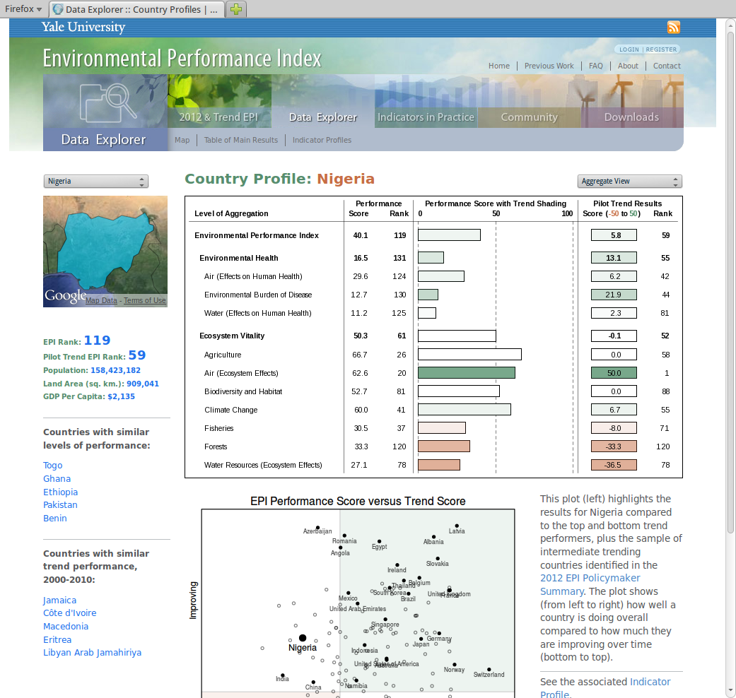 SVG concepts: Hyperlinks
========
SVG concepts: Animation
========
```{r eval=FALSE}
gridsvg("animate.svg", prefix="animate-")
print(latticePlot)
grid.animate("plot_01.xyplot.points.panel.1.1", group=FALSE,
"stroke-opacity"=0:1,
"fill-opacity"=c(0, .2),
duration=mtcars$mpg)
dev.off()
```
```{r echo=FALSE}
# Slightly more complex variation that works a bit better
# but the code looks worse
gridsvg("animate.svg", prefix="animate-")
print(latticePlot)
grid.animate("plot_01.xyplot.points.panel.1.1",
group=FALSE,
"stroke-opacity"=0:1,
"fill-opacity"=c(0, .2),
duration=1 + (mtcars$mpg - min(mtcars$mpg))/5)
dev.off()
```
SVG concepts: Animation
============
SVG concepts: Gradient Fills
========
```{r results="hide"}
gridsvg("gradient-demo.svg", prefix="gradient-demo-")
grid.circle(r=.4, name="circ")
gradient <- radialGradient(c("white", "blue", "black"), fx=.3, fy=.7)
grid.gradientFill("circ", gradient)
dev.off()
```
SVG concepts: Gradient Fills
========
```{r results="hide"}
gridsvg("gradient.svg", prefix="gradient-")
print(latticePlot)
registerGradientFill("specular", gradient)
grid.gradientFill("points", grep=TRUE, group=FALSE,
label=rep("specular", nrow(mtcars)))
dev.off()
```
SVG concepts: Gradient Fills
========
SVG concepts: Gradient Fills
========
SVG concepts: Pattern Fills
========
```{r results="hide"}
gridsvg("pattern-demo.svg", prefix="pattern-demo-")
grid.circle(r=.4, gp=gpar(fill="grey"))
dev.off()
```
SVG concepts: Pattern Fills
========
```{r results="hide"}
barplot <- barchart(table(mtcars$gear),
par.settings=list(background=list(col="grey90")))
```
```{r echo=FALSE}
gridsvg("barchart.svg", prefix="barchart-")
print(barplot)
dev.off()
```
SVG concepts: Pattern Fills
========
```{r results="hide"}
gridsvg("pattern.svg", prefix="pattern-")
print(barplot)
pattern <- pattern(circleGrob(r=.4, gp=gpar(fill="grey")),
width=.05, height=.05)
registerPatternFill("circles", pattern)
grid.patternFill("rect", grep=TRUE, group=FALSE,
label=rep("circles", 3))
dev.off()
```
SVG concepts: Pattern Fills
========
SVG concepts: Filters
========
```{r results="hide"}
gridsvg("filter.svg", prefix="filter-")
print(latticePlot)
blur <- filterEffect(feGaussianBlur(sd=1))
grid.filter("main|lab|tick|border", grep=TRUE, global=TRUE, blur)
dev.off()
```
SVG concepts: Filters
========
SVG concepts: Clipping Paths
============
```{r echo=FALSE}
set.seed(1)
```
```{r results="hide"}
circles <- circleGrob(r=c(.45, .2),
gp=gpar(col=NA, fill=c("grey", "white")))
```
```{r echo=FALSE}
gridsvg("circles.svg", prefix="circles-")
grid.draw(circles)
dev.off()
```
SVG concepts: Clipping Paths
============
```{r results="hide"}
gridsvg("plot-clip.svg", prefix="clip-")
cp <- clipPath(circles)
pushClipPath(cp)
print(latticePlot, newpage=FALSE)
dev.off()
```
SVG concepts: Clipping Paths
============
SVG concepts: Clipping Paths
============
SVG concepts: Clipping Paths
============
SVG concepts: Masks
============
SVG concepts: Masks
============
```{r results="hide"}
gridsvg("plot-masked.svg", prefix="clip-")
mask <- mask(circles)
pushMask(mask)
print(latticePlot, newpage=FALSE)
dev.off()
```
SVG concepts: Masks
============
SVG concepts: Masks
============
SVG concepts: Masks
============
SVG concepts: Masks
============
SVG concepts: Javascript
============
```{r results="hide"}
gridsvg("plot-js.svg", prefix="js-")
print(latticePlot, newpage=FALSE)
grid.garnish("points", grep=TRUE, group=FALSE,
onclick=paste("alert('x =", mtcars$disp,
"y =", mtcars$mpg, "')"))
dev.off()
```
SVG concepts: Javascript
============
SVG concepts: Javascript
============
SVG concepts: Javascript
============
Playing
=======
```{r results="hide"}
gridsvg("leaf.svg", prefix="leaf-")
library(grImport)
leaf <- readPicture("fall12.xml")
grid.picture(leaf)
dev.off()
```
Playing
=======
Playing
=======
Playing
=======
```{r eval=FALSE, echo=FALSE, results="hide"}
outline <- leaf[1]@paths[[1]]
exp <- .05
range <- range(leaf@summary@xscale, leaf@summary@yscale)
xrange <- range + exp*c(-1, 1)*diff(range)
yrange <- xrange
leafvp <- viewport(xscale=xrange, yscale=yrange, name="lvp")
leafGrob <- function(name="leaf", ...) {
pathGrob(x=outline@x, y=outline@y, default="native",
vp=leafvp, name=name, ...)
}
drawLeaf <- function(...) {
grid.draw(leafGrob(...))
}
veinsGrob <- function(name="veins", ...) {
pictureGrob(leaf[-1], exp=0,
xscale=xrange, yscale=yrange,
name=name)
}
drawVeins <- function(...) {
grid.draw(veinsGrob(...))
}
blurAlpha <- feGaussianBlur(input="SourceAlpha",
sd=5, result="blur")
offset <- feOffset(input="blur",
unit(3, "mm"), unit(-3, "mm"))
drop <- filterEffect(list(blurAlpha, offset))
fill <- linearGradient(c("black", "red", "yellow"))
leaf1 <- gradientFillGrob(leafGrob("leaf-1"), fill)
fill2 <- radialGradient(c(rgb(1,0,0,.2), rgb(1,1,0,.4)),
stops=c(0, .7))
pg <- polygonGrob(c(.7, 0, 0, 1, 1),
c(0, .7, 1, 1, 0))
cp <- clipPath(pg)
leaf2 <- clipPathGrob(gradientFillGrob(leafGrob("leaf-2"), fill2), cp)
blur <- filterEffect(feGaussianBlur(sd=1))
veins <- filterGrob(veinsGrob("veins"), blur)
leafTreeChildren <- gList(leaf1, leaf2, veins)
emboss <- filterEffect(list(feConvolveMatrix(kernelMatrix=
rbind(c(1,0,0),
c(0,1,0),
c(0,0,-1)))))
leafTree <- filterGrob(gTree(children=leafTreeChildren), emboss)
shadow <- filterGrob(gradientFillGrob(leafGrob("leaf-shadow"), fill), drop)
leafPattern <- pattern(gTree(children=gList(shadow, leafTree)),
width=.05, height=.05)
registerPatternFill("leaf", leafPattern)
gridsvg("barchart-silly.svg", prefix="silly-")
print(barplot)
grid.patternFill("rect", grep=TRUE, group=FALSE,
label=rep("leaf", 3))
dev.off()
```
```{r eval=FALSE}
gridsvg("barchart-silly.svg", prefix="silly-")
print(barplot)
grid.patternFill("rect", grep=TRUE, group=FALSE,
label=rep("leaf", 3))
dev.off()
```
Summary
=======
* Web publishing (HTML) is hot
* SVG is cool
* gridSVG shows potential
* bringing SVG goodness to R
* bringing R goodness to SVG
Acknowledgements
================
* Many of the new features in 'gridSVG' were implemented by Simon Potter
as part of his Masters Thesis
* The hyperlinked scatterplot example was from Yale's
Environmental Performance Index
* The "Price Kaleidoscope" and "linked map" examples were
produced by David Banks as part of his BSc Honours Project
* The 'lattice' plot with checkboxes and tooltips was
produced by David Banks as part of his Masters Project
* The
leaf image
was created by
OpenClipArt
user
Aungkarn
Sugcharoun
SVG concepts: Hyperlinks
========
SVG concepts: Animation
========
```{r eval=FALSE}
gridsvg("animate.svg", prefix="animate-")
print(latticePlot)
grid.animate("plot_01.xyplot.points.panel.1.1", group=FALSE,
"stroke-opacity"=0:1,
"fill-opacity"=c(0, .2),
duration=mtcars$mpg)
dev.off()
```
```{r echo=FALSE}
# Slightly more complex variation that works a bit better
# but the code looks worse
gridsvg("animate.svg", prefix="animate-")
print(latticePlot)
grid.animate("plot_01.xyplot.points.panel.1.1",
group=FALSE,
"stroke-opacity"=0:1,
"fill-opacity"=c(0, .2),
duration=1 + (mtcars$mpg - min(mtcars$mpg))/5)
dev.off()
```
SVG concepts: Animation
============
SVG concepts: Gradient Fills
========
```{r results="hide"}
gridsvg("gradient-demo.svg", prefix="gradient-demo-")
grid.circle(r=.4, name="circ")
gradient <- radialGradient(c("white", "blue", "black"), fx=.3, fy=.7)
grid.gradientFill("circ", gradient)
dev.off()
```
SVG concepts: Gradient Fills
========
```{r results="hide"}
gridsvg("gradient.svg", prefix="gradient-")
print(latticePlot)
registerGradientFill("specular", gradient)
grid.gradientFill("points", grep=TRUE, group=FALSE,
label=rep("specular", nrow(mtcars)))
dev.off()
```
SVG concepts: Gradient Fills
========
SVG concepts: Gradient Fills
========
SVG concepts: Pattern Fills
========
```{r results="hide"}
gridsvg("pattern-demo.svg", prefix="pattern-demo-")
grid.circle(r=.4, gp=gpar(fill="grey"))
dev.off()
```
SVG concepts: Pattern Fills
========
```{r results="hide"}
barplot <- barchart(table(mtcars$gear),
par.settings=list(background=list(col="grey90")))
```
```{r echo=FALSE}
gridsvg("barchart.svg", prefix="barchart-")
print(barplot)
dev.off()
```
SVG concepts: Pattern Fills
========
```{r results="hide"}
gridsvg("pattern.svg", prefix="pattern-")
print(barplot)
pattern <- pattern(circleGrob(r=.4, gp=gpar(fill="grey")),
width=.05, height=.05)
registerPatternFill("circles", pattern)
grid.patternFill("rect", grep=TRUE, group=FALSE,
label=rep("circles", 3))
dev.off()
```
SVG concepts: Pattern Fills
========
SVG concepts: Filters
========
```{r results="hide"}
gridsvg("filter.svg", prefix="filter-")
print(latticePlot)
blur <- filterEffect(feGaussianBlur(sd=1))
grid.filter("main|lab|tick|border", grep=TRUE, global=TRUE, blur)
dev.off()
```
SVG concepts: Filters
========
SVG concepts: Clipping Paths
============
```{r echo=FALSE}
set.seed(1)
```
```{r results="hide"}
circles <- circleGrob(r=c(.45, .2),
gp=gpar(col=NA, fill=c("grey", "white")))
```
```{r echo=FALSE}
gridsvg("circles.svg", prefix="circles-")
grid.draw(circles)
dev.off()
```
SVG concepts: Clipping Paths
============
```{r results="hide"}
gridsvg("plot-clip.svg", prefix="clip-")
cp <- clipPath(circles)
pushClipPath(cp)
print(latticePlot, newpage=FALSE)
dev.off()
```
SVG concepts: Clipping Paths
============
SVG concepts: Clipping Paths
============
SVG concepts: Clipping Paths
============
SVG concepts: Masks
============
SVG concepts: Masks
============
```{r results="hide"}
gridsvg("plot-masked.svg", prefix="clip-")
mask <- mask(circles)
pushMask(mask)
print(latticePlot, newpage=FALSE)
dev.off()
```
SVG concepts: Masks
============
SVG concepts: Masks
============
SVG concepts: Masks
============
SVG concepts: Masks
============
SVG concepts: Javascript
============
```{r results="hide"}
gridsvg("plot-js.svg", prefix="js-")
print(latticePlot, newpage=FALSE)
grid.garnish("points", grep=TRUE, group=FALSE,
onclick=paste("alert('x =", mtcars$disp,
"y =", mtcars$mpg, "')"))
dev.off()
```
SVG concepts: Javascript
============
SVG concepts: Javascript
============
SVG concepts: Javascript
============
Playing
=======
```{r results="hide"}
gridsvg("leaf.svg", prefix="leaf-")
library(grImport)
leaf <- readPicture("fall12.xml")
grid.picture(leaf)
dev.off()
```
Playing
=======
Playing
=======
Playing
=======
```{r eval=FALSE, echo=FALSE, results="hide"}
outline <- leaf[1]@paths[[1]]
exp <- .05
range <- range(leaf@summary@xscale, leaf@summary@yscale)
xrange <- range + exp*c(-1, 1)*diff(range)
yrange <- xrange
leafvp <- viewport(xscale=xrange, yscale=yrange, name="lvp")
leafGrob <- function(name="leaf", ...) {
pathGrob(x=outline@x, y=outline@y, default="native",
vp=leafvp, name=name, ...)
}
drawLeaf <- function(...) {
grid.draw(leafGrob(...))
}
veinsGrob <- function(name="veins", ...) {
pictureGrob(leaf[-1], exp=0,
xscale=xrange, yscale=yrange,
name=name)
}
drawVeins <- function(...) {
grid.draw(veinsGrob(...))
}
blurAlpha <- feGaussianBlur(input="SourceAlpha",
sd=5, result="blur")
offset <- feOffset(input="blur",
unit(3, "mm"), unit(-3, "mm"))
drop <- filterEffect(list(blurAlpha, offset))
fill <- linearGradient(c("black", "red", "yellow"))
leaf1 <- gradientFillGrob(leafGrob("leaf-1"), fill)
fill2 <- radialGradient(c(rgb(1,0,0,.2), rgb(1,1,0,.4)),
stops=c(0, .7))
pg <- polygonGrob(c(.7, 0, 0, 1, 1),
c(0, .7, 1, 1, 0))
cp <- clipPath(pg)
leaf2 <- clipPathGrob(gradientFillGrob(leafGrob("leaf-2"), fill2), cp)
blur <- filterEffect(feGaussianBlur(sd=1))
veins <- filterGrob(veinsGrob("veins"), blur)
leafTreeChildren <- gList(leaf1, leaf2, veins)
emboss <- filterEffect(list(feConvolveMatrix(kernelMatrix=
rbind(c(1,0,0),
c(0,1,0),
c(0,0,-1)))))
leafTree <- filterGrob(gTree(children=leafTreeChildren), emboss)
shadow <- filterGrob(gradientFillGrob(leafGrob("leaf-shadow"), fill), drop)
leafPattern <- pattern(gTree(children=gList(shadow, leafTree)),
width=.05, height=.05)
registerPatternFill("leaf", leafPattern)
gridsvg("barchart-silly.svg", prefix="silly-")
print(barplot)
grid.patternFill("rect", grep=TRUE, group=FALSE,
label=rep("leaf", 3))
dev.off()
```
```{r eval=FALSE}
gridsvg("barchart-silly.svg", prefix="silly-")
print(barplot)
grid.patternFill("rect", grep=TRUE, group=FALSE,
label=rep("leaf", 3))
dev.off()
```
Summary
=======
* Web publishing (HTML) is hot
* SVG is cool
* gridSVG shows potential
* bringing SVG goodness to R
* bringing R goodness to SVG
Acknowledgements
================
* Many of the new features in 'gridSVG' were implemented by Simon Potter
as part of his Masters Thesis
* The hyperlinked scatterplot example was from Yale's
Environmental Performance Index
* The "Price Kaleidoscope" and "linked map" examples were
produced by David Banks as part of his BSc Honours Project
* The 'lattice' plot with checkboxes and tooltips was
produced by David Banks as part of his Masters Project
* The
leaf image
was created by
OpenClipArt
user
Aungkarn
Sugcharoun