Integrating R Graphics and TikZ Graphics:
The 'dvir' Package
Paul Murrell
The University of Auckland
November 2020
Problem:
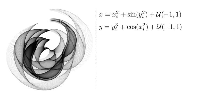
Add a mathematical equation to an R graphics image

Suppose we have an image we have drawn with R and we want to add a mathematical equation to the image. And we want the mathematical equation to look nicer than this sort of ASCII-math approach.
Option 1
R's "plotmath" feature
grid.raster(img, x=0, just="left")
grid.text(expression(x == x[i]^2 - sin(y[i]^2) +
                     italic(U)*group("(", list(-1, 1), ")")))
grid.text(expression(y == y[i]^3 - cos(x[i]^2) +
                     italic(U)*group("(", list(-1, 1), ")")))
One option is to use R's "plotmath" facility. This lets us provide an R expression as an argument to text-drawing functions, like grid.text().
Option 1
- better than nothing
- less than perfect

The expression is interpreted as a mathematical equation and TeX-like rules are used to position the appropriate symbols into something more visually appealing (than ASCII-math).
Option 2
The 'tikzDevice' package
library(tikzDevice)
tikz("tikzMath.tex")
grid.raster(img, x=0, just="left")
grid.text("$x = x_i^2 + \\sin(y_i^2) + {\\mathcal{U}}(-1, 1)$")
grid.text("$y = y_i^3 + \\cos(x_i^2) + {\\mathcal{U}}(-1, 1)$")
dev.off()
Another option is the 'tikzDevice' package. This lets us send TeX expressions to text-drawing functions (provided we are drawing to a tikz() graphics device).
Option 2
- TeX expressions
- TeX output (TeX-quality rendering)
The result is the familiar classy mathematical equation typesetting that we are used to from TeX.
Option 2
The 'tikzDevice' package converts R graphics to TeX
\documentclass[10pt]{article}
\usepackage{tikz}
\begin{document}
\begin{tikzpicture}[x=1pt,y=1pt]
\node[inner] at (  0.00,   0.00) {
  \pgfimage[width=289.08pt,height=289.08pt  ]{tikzMath_ras1}};
\node[] at (289.08,241.24)
  {$x = x_i^2 + \sin(y_i^2) + {\mathcal{U}}(-1, 1)$};
\node[] at (289.08,205.10)
  {$y = y_i^3 + \cos(x_i^2) + {\mathcal{U}}(-1, 1)$};
\end{tikzpicture}
\end{document}
The tikz() graphics device generates a TeX document.
Option 2
TeX can be processed to produce PDF (for example)
pdflatex -fmt pdf tikzMath.tex
That TeX document can be processed, e.g., with pdflatex, to produce a final graphic, e.g., a PDF file.
Option 3
The 'dvir' package
library(dvir)
grid.raster(img, x=0, just="left")
grid.latex("$x = x_i^2 + \\sin(y_i^2) + {\\mathcal{U}}(-1, 1)$")
grid.latex("$y = y_i^3 + \\cos(x_i^2) + {\\mathcal{U}}(-1, 1)$")
The (new) 'dvir' package provides yet another approach. I have a grid.latex() function that I can send TeX expressions.
Option 3
- TeX expressions
- R graphics output (TeX-quality rendering)

'dvir' produces TeX-quality results, just like 'tikzDevice'. The difference is, this is being drawn by R.
Option 3
The 'dvir' package generates TeX ...
\documentclass[12pt]{standalone}
\begin{document}
$x = x_i^2 + \sin(y_i^2) + {\mathcal {U}}(-1, 1)$
\end{document}
... then processes the TeX to produce DVI
pdflatex -fmt dvi dvirMath.tex
'dvir' generates a TeX document and processes it to generate a DVI file.
Option 3
The 'dvir' package converts DVI to R graphics
pre          version=2, num=25400000, den=473628672, mag=1000,
             comment= TeX output 2020.10.14:1528
bop          counters=1 0 0 0 0 0 0 0 0 0, p=-1
y4           a=-1073741823
y0
xxx1         k=32
             x=papersize=141.51582pt,12.51027pt
xxx1         k=51
             x=ps::%%HiResBoundingBox: 0 0 141.51582pt 12.51027pt.
fnt_def_1    fontnum=17, checksum=-1209964637, scale=786432
             fontname=cmmi12
fnt_num_17
set_char_120 'x'
w3           b=218450
'dvir' then reads the DVI file and draws what the DVI file says to draw (where it says to draw it, using the font it says to draw with).
DVI in R Graphics
Now we can read DVI, what else can we do?

Now that we can read DVI files, we can reproduce any TeX output, e.g., TeX tables.
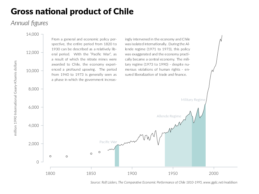
TeX is also quite good at typesetting. This plot contains a set of text typeset into two columns, fully justified, including hyphenation.
DVI in R Graphics
What about TeX graphics ?
\documentclass{standalone}
\usepackage{xcolor}
\usepackage{tikz}
\begin{document}
\pagecolor{white}
\begin{tikzpicture}
\path (0, 2) node[circle,draw](x){A} (4, 0) node[circle,draw](y){B};
\draw (x) .. controls (2, 2) and (2, 0) .. (y);
\end{tikzpicture}
\end{document}
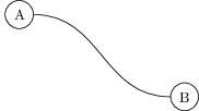
The TikZ package can be used to produce graphics in TeX documents.
TikZ in DVI
TikZ produces "special" PostScript instructions in DVI
xxx1   k=29
       x=ps:: 9.91148 56.69362 moveto
xxx1   k=58
       x=ps:: 56.69362 56.69362 56.69362 0.0 103.60684 0.0 curveto
xxx1   k=12
       x=ps:: pgfstr
A 'dvir' driver for TikZ produces instructions for 'grid'
xxx1   k=86
       x=dvir:: moveto 9.94853,56.90549:
         curveto 56.90549,56.90549,56.90549,0.0,103.99403,0.0:;
xxx1   k=15
       x=dvir:: stroke;
TikZ graphics becomes "special" operations in a DVI file. By default, those special operations contain PostScript code. But the 'dvir' package provides a TikZ driver so that TikZ special operations contain code that 'dvir' can read.
TikZ in R Graphics
'dvir' draws TikZ specials

grid.ls()
GRID.DVIgrob.801
  GRID.gTree.800
    GRID.pathgrob.788
    GRID.text.789
    GRID.pathgrob.795
    GRID.text.796
    GRID.polyline.799
'dvir' takes the TikZ specials in DVI files and converts them to 'grid' drawing.
Integrating R Graphics and TikZ

This is a more complex demonstration of drawing TikZ graphics in R; we have combined a 'ggplot2' plot that contains a smoother with a text label that is drawn along the smoother line using TikZ.
Integrating R Graphics and TikZ

We draw the main plot in R. We export the smoother line from the plot out to TikZ code and add text along the line in TikZ code. We import the label back into R and then edit the colour of the label back in R. An important idea here is "integration". We are not just drawing a picture in another graphics system and including it in an R graphic; we are converting the picture from another graphics system into drawing operations in R; we can then further manipulate the picture within R. This also demonstrates the benefit of ending up back in R; I am happier generating (and allocating) the colours to the TikZ text in R than I would be doing the same thing in TeX/TikZ.
Limitations
- I T I S S L O W
- Only PDF/PostScript and Cairo-based graphics devices (so far).
- Heavyweight system requirements (TeX).
- Only available from github (not CRAN).
Summary
- The 'dvir' package reads DVI output (from TeX) into R graphics
- That is handy for producing TeX-quality mathematical equations
- It also provides access to TeX's general typesetting capabilities
- It even provides access to TeX's (TikZ/PGF) graphics capabilities
Acknowledgements
- Alexander van der Voorn
- TeX
- LuaTeX
- TikZ/PGF
- Katharina Brunner's 'generativeart' package
- The two-column text example is based on Figure 4.1 from Thomas Rahlf's "Data Visualisation with R"
- The global warming data are from NASA