reveal.js

Expanding the Vocabulary of R Graphics

Paul Murrell
The University of Auckland
July 2021

The {ggplot2} package can be used to create data visualisations.

'ggplot2' is an example of an R package that can be used to generate data visualisations. This is my "Bilbo Baggins" slide: start with something simple and uncontroversial that makes people comfortable.

This diagram shows how the 'ggplot2' package fits into the ecosystem of R graphics. The most important feature of this diagram is the 'grDevices' package, which represents the R "graphics engine". The next most important feature is the fact that all other graphics packages pass through 'grDevices' to get to the graphics devices, which produce final output. For example, 'ggplot2' talks to the 'grid' package, which talks to the R graphics engine. This means that the R graphics engine represents a bottle-neck; graphics packages can only do things that the R graphics engine allows them to do. Graphical output is limited to the (limited) vocabulary of the R graphics engine.

The R graphics engine understands rectangles.

'ggplot2' constructs a scatter plot from rectangles ...

The R graphics engine understands lines.

... lines ...

The R graphics engine understands points.

... points ...

The R graphics engine understands text.

... and text.

The {ggplot2} package can be used to create data visualisations.

This is just a repeat of the complete 'ggplot2' plot to show the final result of combining rectangles, lines, points, and text.

The {riverplot} package can be used to create data visualisations.

The 'riverplot' package is another example of an R package that can be used to generate data visualisations. For example, it can be used to draw Sankey diagrams.

Like 'ggplot2', the 'riverplot' package has to go through the R graphics engine to produce output on the graphics devices. In this case, 'riverplot' talks to the 'graphics' package, which talks to the R graphics engine.

How does {riverplot} tell the R graphics engine to draw a gradient fill?

One of the features of the Sankey diagrams that the 'riverplot' package produces is the colour gradient that is used to fill the "edges" in the diagram. The 'riverplot' package must describe this colour gradient using the vocabulary of the graphics engine.

The R graphics engine understands polygons.

the R graphics engine does (did) not understand colour gradients, but it does understand filling polygons with a solid colour. Because of the limitations of the R graphics engine vocabulary, the 'riverplot' package is forced to describe the colour gradient in terms of a series of small polygonal slices, each filled with a slightly different colour.

Could we make the R graphics engine understand gradient fills?

It might make life easier for the 'riverplot' package if the R graphics engine vocabulary included the ability to fill a single polygon with a colour gradient.

A New Vocabulary

So what is new in the R graphics engine for R version 4.1.0? I think you might be able to guess at least part of what is coming ...

From R 4.1.0 it is possible to make use of gradient fills

gradient <- linearGradient(c("white", "transparent"))
grid.rect(gp=gpar(lwd=5, col="white", fill=gradient))

Changes to the R graphics engine in R 4.1.0 mean that the R graphics engine has an expanded vocabulary. One new thing that we can do is to define a linear gradient fill. This means that we can fill a shape with a colour gradient. In this case, we have a gradient that transitions smoothly from white at the bottom-left corner to transparent at the top-right corner. The code shown in this section is just here to make it seem real. We will describe the code interface properly a bit later on.

It is also possible to make use of radial gradients

gradient <- radialGradient(c("white", "transparent"))
grid.rect(gp=gpar(lwd=5, col="white", fill=gradient))

Another new thing that we can do is to define a radial gradient. Again, this means that we can fill a shape with a colour gradient, just a different style of gradient. In this case, we have a gradient that transitions smoothly from white at the centre of the filled region to transparent at the edges.

It is also possible to make use of pattern fills

c <- circleGrob(r=unit(5, "mm"))
pat <- pattern(c, width=unit(15, "mm"), height=unit(15, "mm"),
               extend="repeat")
grid.rect(gp=gpar(fill=pat))

Another new thing we can do is to define a pattern fill. This allows us to fill a shape with a repeating pattern. In this case, we define a pattern consisting of a single filled circle and fill a rectangular region by repeating that circle.

It is also possible to make use of clipping paths

path <- circleGrob(r=.3)
pushViewport(viewport(clip=path))
grid.rect(width=.5, height=.5)

Another new thing we can do is to define a clipping path. This means that we can limit the drawing of one shape to the region bounded by another shape. In this case, we define the clipping path to be a circle, then we draw a filled rectangle. With the clipping path in place, only the part of the rectangle that lies inside the circle is drawn. The significant thing here is that the clipping region is NOT a rectangle. The R graphics engine could always clip to a simple rectangle.

It is also possible to make use of masks

mask <- circleGrob(r=.3, gp=gpar(fill=rgb(1,1,1,.5)))
pushViewport(viewport(mask=mask))
grid.rect(width=.5, height=.5)

The final new thing we can do is to define a mask, or more specifically, a transparency mask. This means that we can define the transparency of one shape based on the transparency of another shape. In this case, we define the mask to be a semi-transparent circle (on a fully transparent background) and we draw a filled rectangle. The transparency of the mask is transferred to the rectangle, so the parts of the rectangle that lie within the circle become semi-transparent and the parts of the rectangle that lie outside the circle become fully transparent. Masking can be viewed as more sophisticated clipping. Or clipping can be viewed as a simple form of masking.

Why a new vocabulary?

What do these new features get us? What can people do with the new R graphics engine vocabulary?

To make it easier for people to do what they want to do, cf. {riverplot}, {ggpattern}, and {ggtextures}.

We have already seen with the 'riverplot' package that there are graphical features that people want to produce even if they have to work quite hard to express what they want to do in terms of the limited R graphics engine vocabulary. There are other packages in the same boat as 'riverplot'. Here we see an example of a pattern fill from the 'ggpattern' package. Like 'riverplot', 'ggpattern' is forced to use polygons to achieve its result and it might benefit from the R graphics engine understanding pattern fills.

To help people to develop ALL of their data visualisations in code.

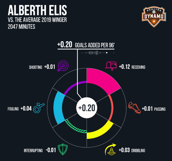
In the case of 'riverplot' and 'ggpattern', when faced with the limitations of the R graphics engine, the solution has been to just work harder to achieve the desired result. Another option, when faced with the limitations of the R graphics engine, is to stop using R and start using something that can do what we want. When this option results in people manually adjusting an image in something like Adobe Illustrator, and NOT producing their image entirely in code, we lose a lot of good things, like reproducibility, version control, sharing, etc ... This image, from the "American Soccer Analysis" web site, is actually an example where the authors have worked very hard to produce the entire result from R code, albeit with some trial-and-error to fine tune the positioning of some elements of the image. Expanding the vocabulary of the R graphics engine can help to make it easier for people to create complete images from R code.

So that R Graphics can speak the same language as other graphics systems, e.g., {grImport}.

R logo R plot with R logo

There are a number of R packages that allow us to import graphics from other systems and draw them as part of an R data visualisation. This can be difficult to achieve if an image from an external system contains a graphical feature that is beyond the limited R graphics engine vocabulary. In this image, on the left, we have the R logo, which contains a subtle colour gradient in both the "hoop" and the "R". On the right, we have added the R logo to a 'ggplot2' scatter plot, INCLUDING the subtle gradient fills.

Who knows what people will do with it?

Expanding the R graphics engine vocabulary expands the expressiveness of the R graphics engine. It is not up to me to figure out what people will try to do with R graphics. This image makes use of masks based on semi-transparency gradients to "fade out" some of the curves. Perhaps the new graphics engine vocabulary will inspire even more creativity from Rtists like Danielle Navarro.

The user interface

In this section, we will look at the new functions in R that provide the user interface for the new graphics vocabulary. We will also look a bit at how these new graphical features are defined and how they work because they may not be familiar to everyone.

The new features are only available so far via a user interface in the {grid} package.

library(grid)

If you want to try out the new R graphics engine vocabulary, for now you will have to work with the interface that is provided by the 'grid' package.

In particular, there is no 'graphics' interface and there is no 'ggplot2' interface (yet). You can retroactively modify 'ggplot2' or 'graphics' data visualisations to add some of the new features, but that requires a good knowledge of 'grid', so we will not address that here; the "Resources" slide has links to documents that include some examples of this sort.

Linear Gradients

We can define a linear gradient with the linearGradient() function.
We can use a linear gradient by specifying it as the value of the fill graphical parameter.

grad <- linearGradient(...)
grid.rect(gp=gpar(fill=grad))

pushViewport(viewport(gp=gpar(fill=grad)))

We use the linearGradient() function to define a linear gradient and then we can provide the resulting object as the value for 'fill' in a call to gpar(). It is possible to fill a single shape or we can make the linear gradient the default fill by specifying it for a viewport.

Linear Gradients

We define a start point and an end point and then colours at "stops" along the line in between.

grad <- linearGradient(c("black", "white", "black"),
                       x1=.25, y1=.5, x2=1, y2=.5,
                       stops=c(0, .5, 1))

A linear gradient is defined by a start point and an end point (indicated by red dots), plus two or more colours at "stops" along the straight line between the end points (indicated by vertical red lines). In this case, the start point is one quarter of the width from the left edge of the region being filled and the end point is at the right edge of the region being filled. There are three stops, one at the start point, one half-way between the start and end points, and one at the end point. The three colours at the three stops are black, white, and black. The region being filled is a rectangle. If the end points are within the limits of the shape that is being filled, we can also control what happens outside the end points (e.g., pad, repeat, invert, ...).

Radial Gradients

We can define a radial gradient with the radialGradient() function.
We can use a radial gradient by specifying it as the value of the fill graphical parameter.

grad <- radialGradient(...)
grid.rect(gp=gpar(fill=grad))

pushViewport(viewport(gp=gpar(fill=grad)))

We use the radialGradient() function to define a radial gradient and then we can provide the resulting object as the value for 'fill' in a call to gpar(). It is possible to fill a single shape or we can make the radial gradient the default fill by specifying it for a viewport.

Radial Gradients

We define a start circle and an end circle and then colours at "stops" along the line in between.

grad <- radialGradient(c("white", "black"),
                       cx1=.8, cy1=.8, r1=.01,
                       cx2=.5, cy2=.5, r2=.5,
                       stops=c(0, 1))

A radial gradient is defined by a start circle and an end circle (indicated by red circles), plus two or more colours at "stops" between the two circles. In this case, the start circle is very small and near the top-right corner of the region being filled and the end circle is the same diameter as and centred on the region being filled. There are just two stops, white at the start circle and black at the end circle. The region being filled is a square.

Fill Patterns

We can define a pattern with the pattern() function.
We can use a pattern by specifying it as the value of the fill graphical parameter.

pat <- pattern(...)
grid.rect(gp=gpar(fill=pat))

pushViewport(viewport(gp=gpar(fill=pat)))

We use the pattern() function to define a pattern and then we can provide the resulting object as the value for 'fill' in a call to gpar(). It is possible to fill a single shape or we can make the pattern the default fill by specifying it for a viewport.

Fill Patterns

We define a pattern by drawing shapes within a subregion of the region that will be filled.

pat <- pattern(circleGrob(r=.1),
               width=.17, height=.17,
               extend="repeat")

A pattern is defined by a 'grid' grob, which describes one or more shapes. We can also specify the size of the pattern within the region that is being filled. In this case, we are defining a pattern based on a single circle (shown by the red circle), but we specify the size of the pattern to be less than the diameter of that circle (shown by the red rectangle). This means that the pattern is actually four small arcs from the perimeter of the circle. We also specify that the pattern repeats within the region being filled and this produces a series of star or diamonds within the filled region.

Clipping paths

We can define a clipping path by specifying a grob as the clip argument on a viewport.

path <- circleGrob()
pushViewport(viewport(clip=path)

We define a clipping path by specifying a 'grid' grob as the value for the 'clip' argument in a 'grid' viewport. This enforces the clipping path until we pop the viewport or push another viewport with another clipping path or with clipping turned off.

Clipping paths

path <- circleGrob(1:2/3, 1:2/3, r=1/5)
pushViewport(viewport(clip=path))
grid.rect(width=.5, height=.5, gp=gpar(fill="black"))

A clipping path is defined by a 'grid' grob, which can be as simple as a single shape, but could also be as complicated as an entire data visualisation. In this case, we have a circle grob that describes two disjoint circles, so the clipping path is the union of the two circular regions (shown by two red circles). When we draw a rectangle filled with black (shown by the red rectangle), the result is just the parts of the filled rectangle that lie within one of the two circles.

Masks

We can define a mask by specifying a grob as the mask argument for a viewport.

mask <- circleGrob()
pushViewport(viewport(clip=mask)

We define a mask by specifying a 'grid' grob as the value for the 'mask' argument in a 'grid' viewport. This enforces the mask until we pop the viewport or push another viewport with another mask or 'NULL' (which represents no mask).

Masks

mask <- circleGrob(1:2/3, 1:2/3, r=1/5,
                   gp=gpar(col=NA, fill=rgb(1,1,1,1:2/2)))
pushViewport(viewport(mask=mask))
grid.rect(width=.5, height=.5, gp=gpar(fill="black"))

A mask is defined by a 'grid' grob, which can be as simple as a single shape, but could also be as complicated as an entire data visualisation. In this case, we have a circle grob that describes two disjoint circles, one with an opaque fill and one with a semi-trasparent fill (shown by two red circles). When we draw a rectangle filled with black (shown by the red rectangle), the opacity of the circles is transferred to the rectangle so the result is just the parts of the filled rectangle that lie within one of the two circles, with one part opaque and the other part semi-transparent.

A mask based on a semi-transparent linear gradient

grad <- linearGradient(c("transparent", "white"), x1=.5, x2=.5)
mask <- rectGrob(gp=gpar(fill=grad))
g <- ggplot(mtcars) + geom_point(aes(disp, mpg))
pushViewport(viewport(mask=mask))
print(g, newpage=FALSE)

The new vocabulary can be combined to produce interesting results. In this case, we define a linear gradient that transitions from transparent at the bottom of the region being filled to white at the top. We then define a mask that is based on a rectangle shape filled with the linear gradient. This produces a mask that transitions from transparent to opaque, from bottom to top. The mask is shown being applied to a 'ggplot2' scatter plot, which becomes more translucent towards the bottom of the scatter plot.

A mask based on a clipping path

path <- circleGrob(1:2/3, r=.25)
mask <- rectGrob(gp=gpar(fill=rgb(1,1,1,.5)),
                 vp=viewport(clip=path))
pushViewport(viewport(mask=mask))
grid.rect(width=.7, height=.7, gp=gpar(fill="white"))

The new vocabulary can be combined to produce interesting results. In this case, we define a clipping path based on two overlapping circles. We then define a mask based on a rectangle shape that is filled with a semi-transparent white and drawn within a viewport that enforces the clipping path. This produces a semi-transparent mask that is the shape of the union of the overlapped circles. The mask is shown being applied to a filled rectangle. The result is just the part of the rectangle that lies within the union of the overlapped circles made semi-transparent.

You can play with the new features using {gggrid}

gradient <- radialGradient(c(NA, "black"))
ggplot(mtcars) + geom_point(aes(disp, mpg)) +
    gggrid::grid_panel(rectGrob(gp=gpar(fill=gradient)))

Although there is no official 'ggplot2' interface to the new R graphics engine vocabulary, the 'gggrid' package (only on GitHub at present) makes it easy to combine the new 'grid' interface with 'ggplot2' data visualisations. In this case, we use the 'grid' interface to define a radial gradient that transitions from transparent at the centre of the region being filled to black at the edges. We then use the grid_panel() function from the 'gggrid' package to add a 'grid' rectangle filled with the radial gradient to the plot region of a 'ggplot2' scatter plot.

This diagram attempts to show how the 'gggrid' package provides a way to combine the 'grid' interface to the new R graphics engine vocabulary with 'ggplot2' data visualisations.

Future Work

This section looks at work that remains to be done. This section could be skipped if there is insufficient time.

The new features are currently implemented for a limited set of graphics devices:

pdf()
Cairo Graphics devices:
- svg()
- cairo_pdf()
- png(type="cairo")
- x11(type="cairo")

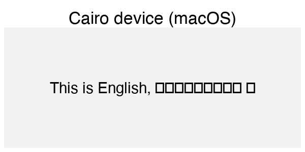
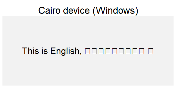
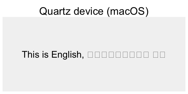
The new R graphics engine vocabulary has only been implemented so far for Cairo-based devices and the pdf() device. All other graphics devices just ignore the new vocabulary.

This diagram attempts to show that only some graphics devices currently support the new R graphics engine vocabulary. Some built-in graphics devices, like the postscript() device, and all third-party graphics devices, like 'ragg', just ignore the new vocabulary.

Support could be added to more graphics devices:

quartz()
postscript()
NOT windows()
The {ragg} package

It would be very useful to expand support for the new R graphics engine vocabulary to more graphics devices. The quartz() device would be a big one for Mac OS users. Support for the 'ragg' device would also be great, given that it is cross-platform and given its importance to the R Studio IDE. NOTE that there is no hope of adding support for the current windows() device for Windows users because the 'graphapp' system upon which the windows() device is built, has its own limited vocabulary. There are a couple of large openings here for contributions from outside of R core!

The vocabulary could be extended further.

circles <- circleGrob(1:2/3, r=.3, gp=gpar(col=NA, fill="white"))
mask <- rectGrob(gp=gpar(col=NA, fill=rgb(1,1,1,.5)))
pushViewport(viewport(mask=mask))
grid.draw(circles)

There are still some things that the new R graphics engine vocabulary does not support. For example, if we apply a mask to a circle grob that describes two overlapping circles, the mask is applied to each circle, one after the other. The result is two overlapping semi-transparent circles, with a visible overlap.

The vocabulary could be extended further.

pushViewport(viewport(mask=mask))
grid.group(circles)

If we extend the R graphics engine vocabulary to include the concept of "isolated" groups, we can produce a different result. Here, the overlapping circles are drawn as a group BEFORE applying the mask. The result now is a semi-transparent version of the result of drawing the two circles. Work on this and related extensions is currently underway.

There will be bugs ...

rects <- rectGrob(x=0:1/2, y=0:1/2, width=1/2, height=1/2,
                  just=c("left", "bottom"),
                  gp=gpar(col=NA, fill=rgb(1,1,1,1:2/2)))
pushViewport(viewport(mask=rects))
grid.rect(gp=gpar(fill=pat))

The new R graphics engine vocabulary has undergone a battery of tests, but not all possible combinations have been explored. In this example, we have a mask consisting of an opaque rectangle and a semi-transparent rectangle being applied to a rectangle filled with a pattern. The result is not as expected because the mask is being applied to the pattern AS WELL AS being applied to the rectangle. The more people use the new R graphics engine vocabulary, the sooner we will find, and hopefully fix, these bugs.

The R Graphics engine does not really understand text. cf. {ragg}.

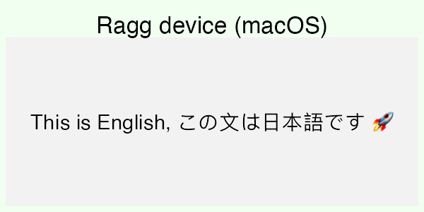
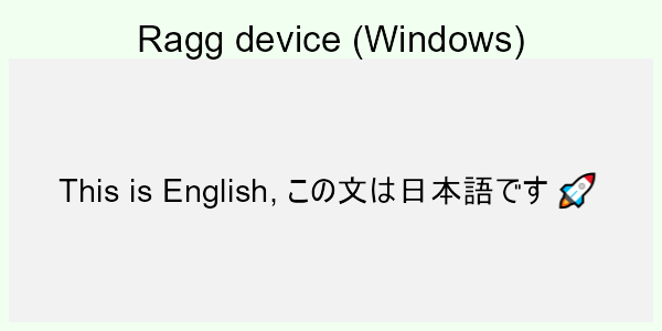
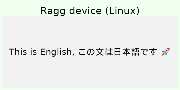
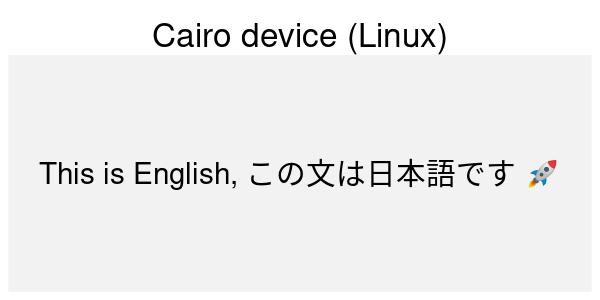
One area where the R graphics engine vocabulary is still severely lacking is in the production of text. The 'ragg' graphics device is leading the way here. Discussions are underway to investigate improvements to the R graphics engine in this area.

Summary

You can now do more things with R Graphics.
Hopefully people will start doing more things.

Acknowledgements

Some of the examples were drawn from the following web sites and R packages.

American Soccer Analysis
The {riverplot} package
The {ggpattern} package
The {ragg} package

Resources

"New Features in the R Graphics Engine"
provides a brief overview.
"Catching up with R Graphics"
provides a detailed description.
"Accessing 'grid' from 'ggplot2'"
describes the {gggrid} package