
This document describes R functions for generating a set of colours and R functions for evaluating a set of colours.
We will make use of the 'colorspace' package and we will show how to use a set of colours with 'ggplot2'.
Colours are often specified in computer code as a red-green-blue
triplet, such as "#FF0000" or rgb(1, 0, 0)
for "red". However, it is more natural and more useful
to describe colour in terms
of three different dimensions: hue, chroma, and luminance (HCL).
Hue corresponds to what we typically call colour, e.g, red, orange,
yellow, green, blue. Chroma describes the purity of the colour,
ranging from very bright/colourful to very dull/grey.
Luminance describes whether the colour is light or dark.
The HCL description of a colour makes it much easier to control the creation of colours. For example, we can create a darker colour just by decreasing the luminance and we can make a brighter colour by increasing the chroma.
The hcl() function in R can be used to specify
a colour in terms of hue, chroma, and luminance.
Hue varies from 0 (red) through green (120) and blue (240)
back to red (360).
Luminance varies from 0 (black) to 100 (white).
Chroma varies from 0 (grey) to 100 (pure).
For example, the following code generates a sequence of blue colours that vary from darker to lighter with constant chroma.
cols <- hcl(240, 50, seq(40, 80, 10), fixup=FALSE)
cols
[1] "#126490" "#3F7CA9" "#5F96C2" "#7DB0DD" "#9ACBF9"
The valid range of chroma and is different for different values of hue and
luminance. By default, invalid values will be "fixed", but this may
produce unexpected results.
Specifying fixup=FALSE will generate
NA colours if the chroma is out of range.
For example, if we naively attempt to span the full range of
luminance values for our blue colours, we get some gaps.
cols <- hcl(240, 50, seq(0, 100, 20), fixup=FALSE)
cols
[1] "#000000" NA "#126490" "#5F96C2" "#9ACBF9" NA

The hcl.colors() function
in the next section works in HCL, but does it cleverly
so that these problems do not arise.
Generating a coherent set of colours is hard, even working in the
HCL colour space with the hcl() function.
It is best to select colours from a set that someone has already
chosen and there are a wide number of good ones to choose from.
Colours are most often used to represent a categorial variable (group membership) and hue is the most useful dimension to use to distinguish between groups. However, we can only use a fairly small number of different hues before they become hard to differentiate.
The palette.colors() function allows us to select
a number of colours from several predefined palettes (sets of colours).
For example, the following code selects the first 5 colours from
the Okabe-Ito palette (which is safe for colour blind viewers).
cols <- palette.colors(5, "Okabe-Ito")
cols
      black      orange     skyblue bluishgreen      yellow
  "#000000"   "#E69F00"   "#56B4E9"   "#009E73"   "#F0E442"

The following code generates the first 5 colours from the "Set 3" palette (a set of light pastel colours from the ColorBrewer project).
cols <- palette.colors(5, "Set 3")
cols
[1] "#8DD3C7" "#FFFFB3" "#BEBADA" "#FB8072" "#80B1D3"

The palette.pals() function lists the full set of
available palettes.
When we want to represent numeric values with colour,
we usually want to vary luminance (dark to light)
and/or chroma (dull to bright and back to dull).
The hcl.colors() function allows us to choose
a number of colours from a large range of predefined palettes.
The simplest palettes hold hue constant and just vary from dark to light (or vice versa). These are called "sequential" palettes. For example, the following code generates 5 shades of green from dark to light.
cols <- hcl.colors(5, "Greens")
cols
[1] "#004616" "#30893B" "#81C07A" "#CAE8C1" "#F6FBF4"

There are slightly more complex multi-hue sequential palettes that also vary hue. For example, the following code generates 5 colours that vary from dark to light and from more blue to more green.
cols <- hcl.colors(5, "GnBu")
cols
[1] "#2F327D" "#0090BA" "#54CABE" "#C7ECD0" "#F5F8EA"

If the values that we are representing have a natural mid-point, like zero, then we may want a "diverging" palette. For example, the following code generates 5 colours that vary from dark blue to white (or light grey) then to dark red.
cols <- hcl.colors(5, "Blue-Red")
cols
[1] "#023FA5" "#A1A6C8" "#E2E2E2" "#CA9CA4" "#8E063B"

The hcl.pals() function lists the full range of palettes
that are available and its type argument can be used to limit
the result to, for example, just "sequential" palettes or just "diverging"
palettes.
It is also possible to use hcl.colors() to select
colours from a "qualitative" palette,
where the colours differ mainly by hue.
This overlaps with the palettes from the palette.colors()
function; the difference with hcl.colors() is that
we can ask for as many colours as we like and the
result is interpolated from the full range of the qualitative palette.
For example, the following code selects 5 colours from the "Set 3"
palette. The result is different from when we used
palette.colors() because that function selected the
first 5 colours from a fixed palette, whereas hcl.colors()
interpolates 5 colours from the full range of colours in the palette.
cols <- hcl.colors(5, "Set 3")
cols
[1] "#FFB3B5" "#CFC982" "#76D9B1" "#85D0F2" "#E7B5F5"

Having generated a set of colours, it is sometimes useful to
be able to tweak them in various ways. For example, the
adjustcolors() function can be used to produce
a semitransparent version of a colour (NOTE the additional pair of
hex characters in the colour descriptions).
adjustcolor(cols, alpha=.5)
[1] "#FFB3B580" "#CFC98280" "#76D9B180" "#85D0F280" "#E7B5F580"
More sophisticated alterations are possible with functions from the
'colorspace' package: lighten(), darken(),
and desaturate (reduce chroma). For example, the
following code produces a darker version of the palette above.
darker <- colorspace::darken(cols, .2)
darker
[1] "#DC8285" "#A39E58" "#4FAC88" "#57A4C4" "#C086D0"

The 'colorspace' package provides functions for checking how a set of colours will perform when printed in greyscale and when viewed by people with a colour vision deficiency (CVD).
library(colorspace)
The desaturate() function converts colours to greyscale.
cols <- hcl.colors(5, "Greens")
cols
[1] "#004616" "#30893B" "#81C07A" "#CAE8C1" "#F6FBF4"

greys <- desaturate(cols)
greys
[1] "#3B3B3B" "#787878" "#B1B1B1" "#DFDFDF" "#F9F9F9"

The deutan() and protan() functions
simulate the appearance of colours for the most common
forms of CVD (deuteranomaly or protananomaly).
This allows us to check whether a palette that we have generated
contains colours that will appear indistinguishable for
people with CVD.
cols <- palette.colors(5, "Okabe-Ito")
cols
      black      orange     skyblue bluishgreen      yellow
  "#000000"   "#E69F00"   "#56B4E9"   "#009E73"   "#F0E442"

nogreen <- deutan(cols)
nogreen
[1] "#000000" "#DDAB04" "#859CE8" "#6D6F76" "#FFDF46"

When we use the 'ggplot2' package to create a data visualisation,
and we are mapping a variable to the colour aesthetic,
and we want to control the selection of colours,
the easiest thing to do is to manually specify the colour scale
with scale_colour_manual().
For example, the following code generates three colours from the Okabe-Ito palette and uses those to colour the dots in a scatter plot.
library(ggplot2)
cols <- palette.colors(4, "Okabe-Ito")[-1]
ggplot(mpg) +
    geom_point(aes(x = displ, y = cty, colour = drv)) +
    scale_colour_manual(values = unname(cols))
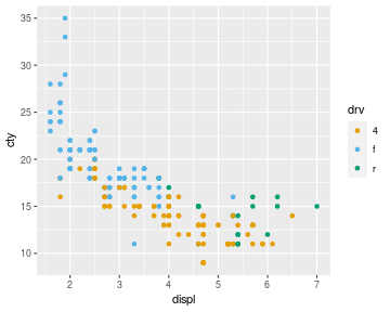
A small detail in the code above is
that we have to use unname()
to get rid of the names on the vector of colours that is generated
by palette.cols(); that is
not necessary when we generate colours with hcl.colors().
The Section on "Replacing a scale" from "R for Data Science" also discusses the problem of replacing a 'ggplot2' colour scale.
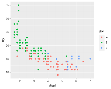
Sometimes we may want to reproduce the set of colours that
'ggplot2' has chosen for us. This can be tricky and may require
a journey through the help pages of 'ggplot2'. For example,
suppose we map a categorical variable to the colour
aesthetic as shown below. Where do those three colours come from ?
ggplot(mpg) +
    geom_point(aes(x = displ, y = cty, colour = drv))
We are looking for a scale that maps a categorical variable to colour.
So we could try the help page ?scale_colour_discrete.
That immediately tells us that this defaults to
?scale_colour_hue. That help page talks about a "palette
function", e.g., ?scales::hue_pal (from the 'scales'
package) and the examples on that page show us what to do.
cols <- scales::hue_pal()(3)
cols
[1] "#F8766D" "#00BA38" "#619CFF"

Another option is to use the 'gggrid' package to print out the colours that 'ggplot2' has used. However, notice that this may return the colours in a different order.
library(gggrid)
ggplot(mpg) +
    geom_point(aes(x = displ, y = cty, colour = drv)) +
    grid_panel(mapping = aes(colour = drv),
               debug = function(data, coords) print(unique(data$colour)))
[1] "#00BA38" "#F8766D" "#619CFF"
