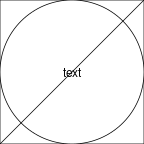
grid.rect()
grid.circle()
grid.segments()
grid.text("text")
This document provides an overview of the main ideas in the 'grid' graphics system.
library(grid)
The 'grid' package provides functions for drawing simple shapes,
like rectangles
(grid.rect()),
circles
(grid.circle()),
straight line segments
(grid.segments),
and text
(grid.text).
By default, these shapes are centred on and/or are the full size of the image.
grid.rect() grid.circle() grid.segments() grid.text("text")
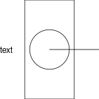
Arguments like x, y,
width, and height allows us to
specify precise locations and dimensions, by default as
proportions of the image dimensions.
By default, shapes are centred on their location,
but a just argument allows us to specify a justification,
like "left" for left-justified.
grid.rect(width = .5)
grid.circle(r = .2)
grid.segments(x0 = .5, y0 = .5, x1 = 1, y1 = .5)
grid.text("text", x = 0, just = "left")
Other shapes include straight lines through multiple points
(grid.lines()),
data symbols
(grid.points()),
polygons
(grid.polygon()),
and raster images
(grid.raster()).
We can position shapes using a variety of coordinate systems. The default is usually "npc", where (0, 0) is the bottom-left corner and (1, 1) is the top-right corner.
Other possibilities include millimetres
("mm"),
inches
("in"),
and lines of text
("lines").
We associate a value with a coordinate system using the
unit() function.
We can also use simple arithmetic on units.
grid.rect(width=unit(.5, "npc"), height=unit(.5, "npc"))
grid.circle(unit(1, "npc") - unit(.5, "in"),
            unit(1, "npc") - unit(.5, "in"),
            unit(.5, "in"))
grid.segments(.1, .1, .9, .9)
grid.text("text", y=.2)
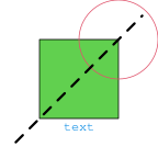
We can control the appearance of the shapes, things like
(border and fill) colour, line type and line width,
and font settings, using the gp
argument and the gpar() function.
grid.rect(width=unit(.5, "npc"), height=unit(.5, "npc"),
          gp=gpar(fill=3))
grid.circle(unit(1, "npc") - unit(.5, "in"),
            unit(1, "npc") - unit(.5, "in"),
            unit(.5, "in"),
            gp=gpar(col=2, fill=NA))
grid.segments(.1, .1, .9, .9,
              gp=gpar(lty="dashed", lwd=3))
grid.text("text", y=.2,
          gp=gpar(fontfamily="mono", col=4))
See the help page for gpar for a complete list of
graphical parameters and the values that they can take.
In the above example, we have specified colours using a simple integer,
which selects a colour from the default colours palette
(see ?palette). We have also specified a generic
monospace font (with "mono").
Later topics will go into the selection of colours and fonts in
more detail.
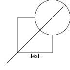
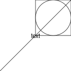
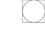
We can create viewports, which are rectangular regions with their own coordinate systems. When we "push" a viewport, all drawing is relative to that viewport until we navigate "up" out of the viewport.
In the following code, we draw exactly the same shapes as in the very first example, but we draw the rectangle and the circle within a viewport that occupies just the top-right quarter of the image. This means that the rectangle and the circle only occupy the top-right quarter of the image (rather than the whole image). The line segment and the text are drawn after we have navigated up from the viewport, back to the entire image, so they still occupy (or are centred on) the entire image).
vp <- viewport(x=1, y=1, width=.5, height=.5,
               just=c("right", "top"))
pushViewport(vp)
grid.rect()
grid.circle()
upViewport()
grid.segments()
grid.text("text")
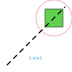
The following code repeats another example from the
Graphical parameters section,
this time the example that positions the shapes using a variety of
coordinate systems (and graphical parameter settings).
We again drawing the rectangle and circle within a viewport in the
top-right quarter of the image. Compared to the original example,
the rectangle is shifted
up into the top-right corner because it is positioned using the
default "npc" coordinates; originally it was half the width and half the
height of the whole image, but now it is half the width and half
the height of the viewport. On the other hand,
the circle appears in the same
place as it did in the original example
because it is located relative to the top-right
corner of the viewport (and the top-right corner of the viewport
is the same as the top-right corner of the image) and because
the radius of the circle is in inches, which are the same in
all viewports.
The text and the line segment are the same as in the
Graphical parameters section because they are
drawn after the upViewport() call, so they are
positioned relative to the entire image.
vp <- viewport(x=1, y=1, width=.5, height=.5,
               just=c("right", "top"))
pushViewport(vp)
grid.rect(width=unit(.5, "npc"), height=unit(.5, "npc"),
          gp=gpar(fill=3))
grid.circle(unit(1, "npc") - unit(.5, "in"),
            unit(1, "npc") - unit(.5, "in"),
            unit(.5, "in"),
            gp=gpar(col=2, fill=NA))
upViewport()
grid.segments(.1, .1, .9, .9,
              gp=gpar(lty="dashed", lwd=3))
grid.text("text", y=.2,
          gp=gpar(fontfamily="mono", col=4))
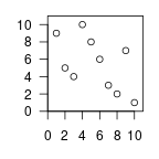
We can define an x-axis scale
(xscale)
and a y-axis scale
(yscale)
for a viewport. This defines a "native"
coordinate system for the viewport, which
is convenient for drawing shapes that represent data
values.
In the code below, we draw a simple scatterplot. We position circles within the plot (for data symbols) by setting up scales on a viewport and then drawing the circles relative to the "native" scales of the viewport.
x <- 1:10
y <- sample(1:10)
x
[1] 1 2 3 4 5 6 7 8 9 10
y
[1] 9 5 4 10 8 6 3 2 7 1
vp <- viewport(x=unit(3, "lines"), y=unit(3, "lines"),
               width=unit(1, "npc") - unit(4, "lines"),
               height=unit(1, "npc") - unit(4, "lines"),
               just=c("left", "bottom"),
               xscale=c(0, 11),
               yscale=c(0, 11))
pushViewport(vp)
grid.rect()
grid.circle(unit(x, "native"),
            unit(y, "native"),
            unit(1, "mm"))
grid.xaxis()
grid.yaxis()
upViewport()
When we draw a shape, we actually create a graphical object, or grob, that describes the shape, and then we draw the grob.
grid.rect()
grid.circle()

We can list the current grobs in an image.
grid.ls()
GRID.rect.31
GRID.circle.32
Instead of immediately drawing a shape, we can just create
a grob that describes the shape - for each grid.*()
function, there is a *Grob() function as well.
This allows us to create a description of what we want to draw
separately from drawing it.
r <- rectGrob()
c <- circleGrob()
The grid.draw() function can be used to draw a grob.
grid.draw(r)
grid.draw(c)

We can create a collection of shapes to draw by combining them as a "tree" of grobs - a gTree.
gt <- gTree(children = gList(r, c))
When we draw a gTree, we draw all of the "children" of the gTree.
grid.draw(gt)
We can also include a viewport in the gTree description. When the gTree is drawn, the viewport is pushed first, which means that the children of the gTree are drawn within the viewport.
vp <- viewport(x = 1, y = 1, just = c("right", "top"),
               width = .5, height = .5)
gt <- gTree(children = gList(r, c), vp = vp)
grid.draw(gt)
This allows us to create an object that describes a collection of objects to draw, including viewports to draw them within. Being able to create grobs and gTrees is useful when we want to provide shapes for other functions to draw (as in the next section).
This section describes how to combine 'grid' drawing with a 'ggplot2' plot.
library(ggplot2)
The 'gggrid' package provides functions that allow us to add 'grid' grobs to a 'ggplot2' plot.
library(gggrid)
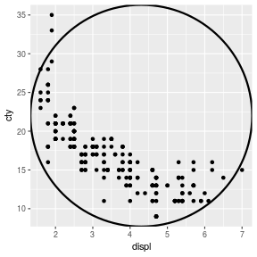
The grid_panel() function draws a 'grid' grob
within the plot region of a 'ggplot2' plot.
Notice that the circle is centred on (and fills) the (grey) plot region
of the 'ggplot2' plot (i.e., it is drawn within a viewport that represents
the plot region).
ggplot(mpg) +
    geom_point(aes(x = displ, y = cty)) +
    grid_panel(circleGrob(gp=gpar(lwd=3, fill=NA)))
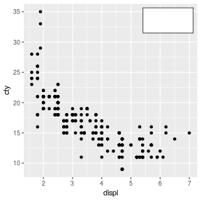
This allows us to add low-level 'grid' drawing to a high-level
'ggplot2' plot. For example, the following code positions
a rectangle precisely 2mm in from the top-right corner
within a 'ggplot2' plot
using the 'grid' unit() function.
r <- rectGrob(x = unit(1,"npc") - unit(2, "mm"),
              y = unit(1,"npc") - unit(2, "mm"),
              width = unit(1, "in"),
              height = unit(.5, "in"),
              just = c("right", "top"))
ggplot(mpg) +
    geom_point(aes(x = displ, y = cty)) +
    grid_panel(r)
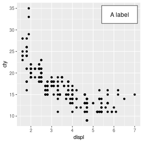
We can draw several shapes by providing a gTree to draw. The following code describes a viewport in the top-right corner of the plot region, plus a rectangle and a text label, then creates a gTree that will draw both the rectangle and the text within the viewport.
vp <- viewport(x = unit(1,"npc") - unit(2, "mm"),
               y = unit(1,"npc") - unit(2, "mm"),
               width = unit(1, "in"),
               height = unit(.5, "in"),
               just = c("right", "top"))
r <- rectGrob()
t <- textGrob("A label")
gt <- gTree(children = gList(r, t), vp = vp)
ggplot(mpg) +
    geom_point(aes(x = displ, y = cty)) +
    grid_panel(gt)
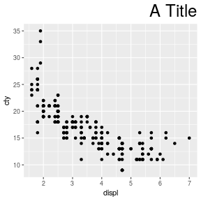
It is also possible to draw a 'ggplot2' plot within a 'grid' image.
Like with 'grid' drawing functions, the ggplot()
function in 'ggplot2' creates a "ggplot" object, which is
automatically drawn. However, we can assign the result of
a ggplot() call to a symbol and just get the
"ggplot" object without drawing the plot.
This allows us to draw the plot later.
For example, the following code
creates a "ggplot" object g,
then pushes a 'grid' viewport (that only occupies the
bottom .9 of the image) and draws g
within that viewport.
We then navigate up out of the viewport and use
'grid' to draw a title at the to of the image.
g <- ggplot(mpg) +
         geom_point(aes(x = displ, y = cty))
pushViewport(viewport(y = 0, height = .9, just = "bottom"))
plot(g, newpage = FALSE)
upViewport()
grid.text("A Title",
          x = unit(1,"npc") - unit(2, "mm"),
          y = unit(1,"npc") - unit(2, "mm"),
          just = c("right", "top"), gp = gpar(cex = 2))