Introduction
Introduction
Where is grid ?

Where is grid ?
  library(lattice)
  xyplot(mpg ~ disp, mtcars)

Exploring grid Grobs
Exploring grid Grobs
grid Viewports
xyplot(mpg ~ disp, mtcars)

Exploring grid Viewports
Exploring grid Viewports
Exploring grid Viewports
Exploring grid Viewports
Exercise
Why Grobs ?
library(lattice)
barchart(Party ~ Amount_Donated, sortedTotals)

Why Grobs ?
Why Grobs ?
library(grid)
grid.remove("plot_01.border.panel.1.1")

Working With Grobs
Modifying Grobs
Modifying Grobs
library(grid)
grid.edit("plot_01.ticklabels.bottom.panel.1.1",
  just=c("left", "top"))

Modifying Grobs
Modifying Grobs
Modifying Grobs
library(grid)
grid.edit("plot_01.ticklabels.bottom.panel.1.1",
  gp=gpar(col="grey"))

Exercise
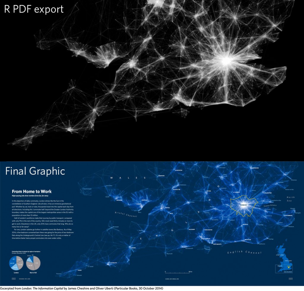
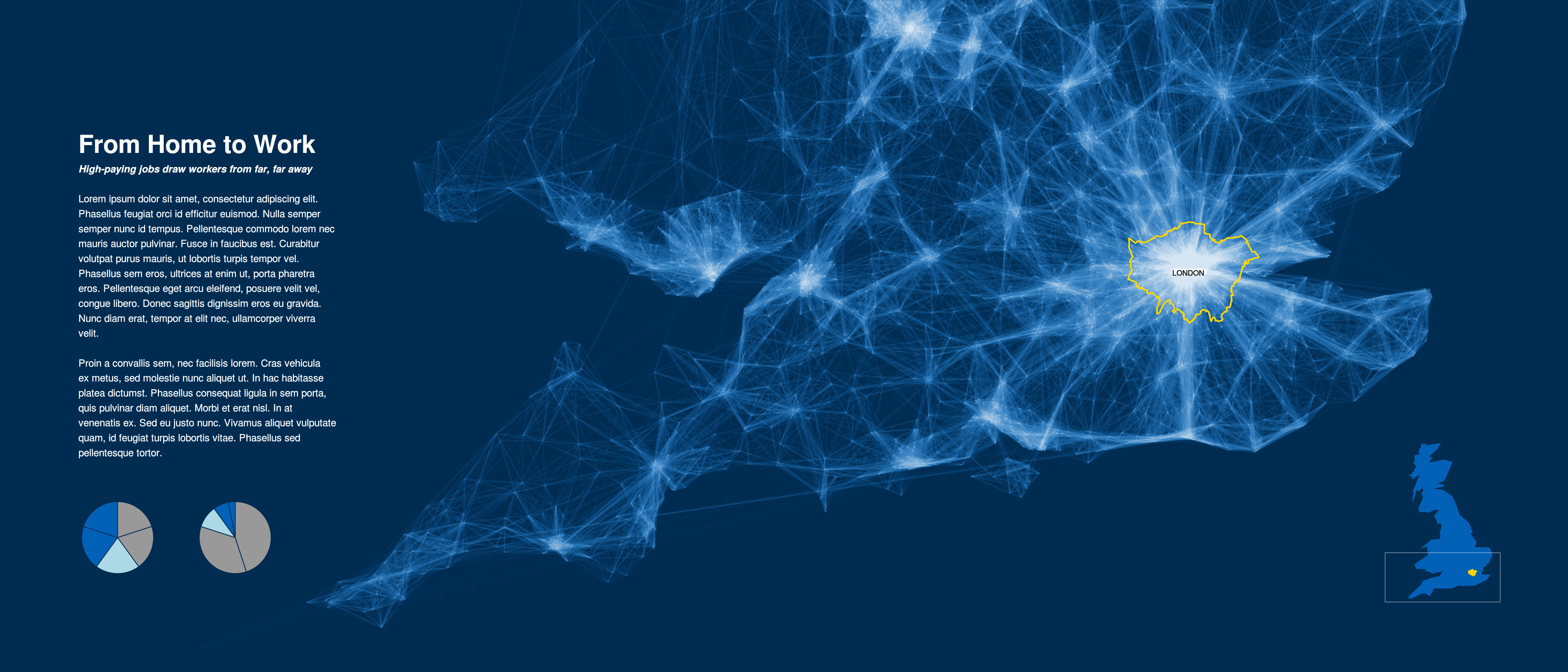
Why Viewports ?
Credit: John G. Bullock, Yale University.
Why Viewports ?
Credit: John G. Bullock, Yale University.
Navigating Viewports
xyplot(mpg ~ disp, mtcars)
Navigating Viewports
Navigating Viewports

Navigating Viewports
downViewport("plot_01.toplevel.vp")
grid.rect(gp=gpar(col=NA, fill=rgb(0,1,0,.5)))

Navigating Viewports
downViewport("plot_01.panel.1.1.vp")
grid.rect(gp=gpar(col=NA, fill=rgb(1,0,0,.5)))

Navigating Viewports
upViewport()
grid.rect(gp=gpar(col=NA, fill=rgb(0,0,1,.5)))

Exercise
Exercise
This is the result you are looking for:

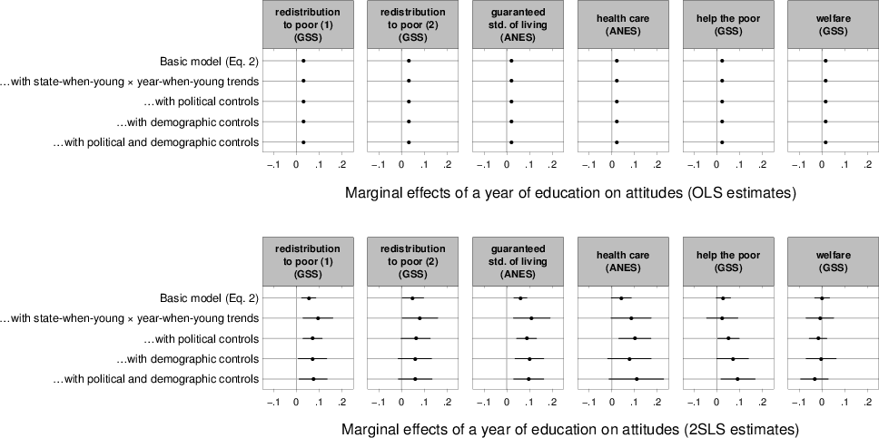
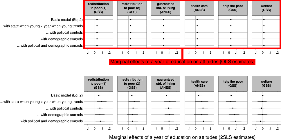
Why Viewports ?
Credit: Pascal A. Niklaus, University of Zurich.
Why Viewports ?
Credit: Pascal A. Niklaus, University of Zurich.
Why Viewports ?
Credit: Brad Boehmke.
Viewport Coordinates
xyplot(mpg ~ disp, mtcars)
downViewport("plot_01.panel.1.1.vp")
Viewport Coordinates
grid.text("native",
  x=unit(300, "native"), y=unit(30, "native"),
  just=c("left", "bottom"))

Viewport Coordinates
grid.text("absolute",
  x=unit(1, "in"), y=unit(1, "cm"),
  just=c("left", "bottom"))

Viewport Coordinates
grid.text("normalised",
  x=unit(.75, "npc"), y=unit(.5, "npc"),
  just=c("left", "bottom"))

Viewport Coordinates
grid.text("normalised - absolute",
  x=unit(1, "npc") - unit(1, "cm"),
  y=unit(1, "npc") - unit(1, "cm"),
  just=c("right", "top"))

Drawing Grobs
Drawing Grobs
grid.rect(x=unit(.2, "npc"), y=unit(100, "native"),
  width=unit(1, "in"), height=unit(1, "lines"))

Drawing Grobs
grid.circle(x=1:5/6, y=.5, r=1:5/25)

Exercise
Exercise
This is the result you are looking for:

Why Viewports ?
Credit: Tom Wright, affiliation unknown.
Why Viewports ?

Why Viewports ?

Starting a New Page
grid.newpage()

Creating Viewports
vp <- viewport(width=.5, height=.5)
pushViewport(vp)
grid.rect(gp=gpar(col=NA, fill="grey80"))

Creating Viewports
vp2 <- viewport(x=0, y=.5, width=.5, height=.5,
        just=c("left", "bottom"))
pushViewport(vp2)
grid.rect()

Creating Viewports
grid.newpage()
pushViewport(vp)
print(xyplot(mpg ~ disp, mtcars), newpage=FALSE)

Exercise
Exercise
This is the result you are looking for:

Summary
Where is grid ?
library(ggplot2)
qplot(disp, mpg, data=mtcars, main="Fast Cars")

Exploring grid Grobs
Modifying Grobs
grid.edit("title.2-4-2-4", gp=gpar(col="red"))

Modifying Grobs
grid.remove("title.2-4-2-4")

Modifying Grobs
Navigating Viewports
Navigating Viewports
downViewport("panel.3-4-3-4")
grid.rect(gp=gpar(col=NA, fill=rgb(0,1,0,.5)))

Exercise
Exercise
This is the result you are looking for:

Where is grid ?
library(vcd)
mosaic(Titanic)

Exploring grid Grobs
Where is grid ?

Where is grid ?
plot(mpg ~ disp, mtcars, pch=16, main="Fast Cars")
library(gridGraphics)
grid.echo()

Exploring grid Grobs
Navigating Viewports
Exercise
Exercise
This is the result you are looking for (before you delete the title):

Why grid ?

Why grid ?

Why grid ?

Why grid ?
grid Layouts

Creating Layouts
widths <- unit(c(1, 2, 1), c("null", "null", "cm"))
lay <- grid.layout(3, 3, widths=widths)
vplay <- viewport(layout=lay)
pushViewport(vplay)
pushViewport(viewport(layout.pos.row=2,
              layout.pos.col=2))
grid.rect(gp=gpar(col=NA, fill=rgb(1,0,0,.5)))

Exercise
Exercise
This is the result you are looking for (the grid.show.layout() function takes a 'grid' layout as its argument and draw a diagram of the layout):

Viewport Coordinates
grid.rect(width=stringWidth("axis label"))

Viewport Coordinates
grid.text("axis label", name="t")
grid.rect(width=grobWidth("t"))

Why grid ?
Viewport Coordinates
grid.text("label", x=1/3, y=1/3, name="t")
grid.circle(2/3, 2/3, r=unit(1, "mm"),
    gp=gpar(fill="black"))
grid.segments(grobX("t", 0), grobY("t", 0), 2/3, 2/3)

Exercise
Exercise
This is the result you are looking for:

Why grid ?

Where is grid ?
gridSVG
library(gridSVG)
grid.circle(r=.2, name="c")
grid.filter("c", filterEffect(feGaussianBlur(sd=3)))
grid.export()

Exercise
Exercise
This is the result you are looking for
(which is an
SVG file):
