<?xml version="1.0" encoding="UTF-8"?>
<html>
  <head>
    <style type="text/css">
    @media print {
      body { }
      p.img { text-align: center; page-break-inside: avoid }
      img.CC { display: inline }
    }
    @media screen {
      body { max-width: 800px; margin: auto }
      p.img { text-align: center }
      img.CC { display: inline }
    }
    p.date {
      font-size: smaller;
      margin: 0;
    }
    p.ref {
      text-indent: -2em;
      padding-left: 2em;
    }
  </style>
    <!-- Google Analytics tracking code -->
    <script>
  (function(i,s,o,g,r,a,m){i['GoogleAnalyticsObject']=r;i[r]=i[r]||function(){
  (i[r].q=i[r].q||[]).push(arguments)},i[r].l=1*new Date();a=s.createElement(o),
  m=s.getElementsByTagName(o)[0];a.async=1;a.src=g;m.parentNode.insertBefore(a,m)
  })(window,document,'script','https://www.google-analytics.com/analytics.js','ga');

  ga('create', 'UA-88814550-1', 'auto');
  ga('send', 'pageview');

  </script>
  </head>
  <body>
    <h1>Variable-Width Lines in R</h1>
    <p>
      <span style="font-style: italic">by Paul Murrell</span>
      <a href="http://orcid.org">
        <img alt="" src="https://www.stat.auckland.ac.nz/~paul/ORCID/ORCiD.png" style="width: 16px; height: 16px; vertical-align: middle"/>
      </a>
      <span style="font-family: mono; font-size: small">
        <a href="http://orcid.org/0000-0002-3224-8858">http://orcid.org/0000-0002-3224-8858</a>
      </span>
    </p>
    <p class="date">
      <rcode echo="FALSE" results="asis"><![CDATA[
cat(format(Sys.Date(), "%A %d %B %Y"))
    ]]></rcode>
    </p>
    <rcode id="init" echo="FALSE" message="FALSE" results="hide"><![CDATA[
opts_chunk$set(comment=" ", tidy=FALSE)

mysvg <- function(filename, width, height) {
    svg(filename, width, height, bg="transparent")
}
  ]]></rcode>
    <hr/>
    <p><a rel="license" href="http://creativecommons.org/licenses/by/4.0/"><img class="CC" alt="Creative Commons License" style="border-width:0" src="https://i.creativecommons.org/l/by/4.0/88x31.png"/></a><br/><span xmlns:dct="http://purl.org/dc/terms/" property="dct:title">This document</span>
    is licensed under a <a rel="license" href="http://creativecommons.org/licenses/by/4.0/">Creative
    Commons Attribution 4.0 International License</a>.
  </p>
    <hr/>
    <!--
  <p style="color: red">
    FIXME: add "how to cite this document" at end
  </p>
  <p style="color: red">
    Add version tag to vwline on github
    git tag v0.1
    git push origin v0.1
  </p>
  <p style="color: red">
    FIXME: need to create Docker image pmur002/power-curve
  </p>
  <p style="color: red">
    FIXME: once Docker image is ready, need to build using 'make docker'
  </p>
  <p style="color: red">
    FIXME: once document is building with 'make docker', need to push
    pmur002/power-curve to Docker Hub
  </p>
  -->
    <p>
    This document describes the 'vwline' package, which provides
    an R interface for drawing variable-width
    curves.  The package provides functions to draw line
    segments through a set of locations, or a smooth curve relative
    to a set of control points, with the width of the line allowed
    to vary along the length of the line.
  </p>
    <div>
      <h2>Table of Contents:</h2>
      <ul>
        <li>
          <a href="#intro">Introduction</a>
        </li>
        <li>
          <a href="#method-1">Method 1: Offsetting points</a>
        </li>
        <li>
          <a href="#method-2">Method 2: Offsetting control points</a>
        </li>
        <li>
          <a href="#method-3">Method 3: Offsetting line segments</a>
        </li>
        <li>
          <a href="#method-4">Method 4: Sweeping curves with a brush</a>
        </li>
        <li>
          <a href="#method-4">Method 5: Offsetting curves</a>
        </li>
        <li>
          <a href="#Detail">Fine tuning variable-width lines</a>
        </li>
        <li>
          <a href="#Gallery">A gallery of variable-width lines</a>
        </li>
        <li>
          <a href="#Discussion">Discussion</a>
        </li>
        <li>
          <a href="#Requirements">Technical requirements</a>
        </li>
        <li>
          <a href="#Resources">Resources</a>
        </li>
        <li>
          <a href="#references">References</a>
        </li>
      </ul>
    </div>
    <h2>
      <a name="intro">Introduction</a>
    </h2>
    <p>
    This document describes the 'vwline' package for drawing variable-width
    curves in R.  For example, of the three lines shown below, standard R
    graphics can draw lines A and B (a line between two points, with a constant
    width) but not line C (a line between two points with a variable width).
  </p>
    <rcode message="FALSE"><![CDATA[
library(grid)
library(vwline)
  ]]></rcode>
    <rcode id="lines" echo="FALSE" fig.keep="none" results="hide"><![CDATA[
svg("figure/lines.svg", width=3, height=3, bg="transparent")
grid.rect(gp=gpar(col=NA, fill="grey90"))
grid.text(LETTERS[3:1], .1, c(.2, .5, .8), gp=gpar(cex=2))
grid.lines(c(.2, .9), .8)
grid.lines(c(.2, .9), .5, gp=gpar(lwd=20, lineend="butt"))
## FIXME: this could just be a grid.brushline()
## grid.brushline(verticalBrush, c(.2, .9), .2, w=c(0, .1))
# grid.brushXspline(verticalBrush, c(.2, .9), rep(.2, 2), 
#                   w=widthSpline(c(0, .2), shape=0))
grid.vwcurve(c(.2, .9), .2, c(0, .1))
dev.off()
  ]]></rcode>
    <p class="img">
      <img src="figure/lines.svg" width="30%"/>
    </p>
    <p>
    It is possible in R graphics to draw line C as
    a filled polygon, by explicitly specifying the outline of the 
    line boundary. For example, in this case the boundary is just a triangle.  
    Several R packages provide functions for drawing polygons of this
    sort, where the boundary is completely specified from data, or
    the boundary can be easily calculated from data as a simple
    x-shift or y-shift. Examples include 
    <code>geom_ribbon</code> (and <code>geom_smooth</code>) in 'ggplot2', 
    <code>kiteChart</code> in 'plotrix', and
    the variations on "violin plots"
    in the 'beanplot' package.
  </p>
    <rcode id="geom-smooth" echo="FALSE" dev="svg" fig.width="3" fig.height="3" out.width="300px" include="FALSE"><![CDATA[
library(ggplot2)
ggplot(mpg, aes(displ, hwy)) +
       geom_point() +
       geom_smooth()
  ]]></rcode>
    <rcode id="kitechart" echo="FALSE" dev="svg" fig.width="3" fig.height="3" out.width="300px" include="FALSE"><![CDATA[
library(plotrix)
musicmat<-matrix(c(c(0.5,0.4,0.3,0.25,0.2,0.15,0.1,rep(0.05,44))+runif(51,0,0.05),
       c(0.1,0.2,0.3,0.35,0.4,0.5,0.4,rep(0.5,14),rep(0.4,15),rep(0.3,15))+runif(51,0,0.1),
       rep(0.15,51)+runif(51,0,0.1),
       c(rep(0,29),c(0.1,0.2,0.4,0.5,0.3,0.2,rep(0.05,16))+runif(22,0,0.05)),
       c(rep(0,38),c(rep(0.05,6),0.08,0.15,0.20,0.25,0.2,0.25,0.3)+runif(13,0,0.05))),
       ncol=51,byrow=TRUE)
kiteChart(musicmat,ann=FALSE, varlabels=rep("", 5),
       timepos=0,timelabels="",mar=rep(2, 4))
  ]]></rcode>
    <rcode id="beanplot" echo="FALSE" dev="svg" fig.width="3" fig.height="3" out.width="300px" include="FALSE"><![CDATA[
library(beanplot)
par(mar=rep(2, 4))
beanplot(list(all = ToothGrowth$len), len ~ supp, ToothGrowth, len ~ dose,
         axes=FALSE)
box()
  ]]></rcode>
    <p class="img">
      <img src="figure/geom-smooth-1.svg" width="30%"/>
      <img src="figure/kitechart-1.svg" width="30%"/>
      <img src="figure/beanplot-1.svg" width="30%"/>
    </p>
    <p>
    However, in situations where the line itself is not simple and
    the width is not just an x-shift or y-shift calculation, the 
    description of the boundary can be much less straightforward.
    In the example below, the line is an 
    <a href="#blanc+schlick">X-spline</a>, which R can
    draw as a line with constant width (lines D and E), but when the 
    width of the line is allowed to vary, standard R graphics cannot
    help, and it is not straightforward to represent the line as 
    a polygon because 
    the boundary becomes a non-trivial path
    (line F).
  </p>
    <rcode id="curves" echo="FALSE" fig.keep="none" results="hide"><![CDATA[
svg("figure/curves.svg", width=3, height=3, bg="transparent")
grid.rect(gp=gpar(col=NA, fill="grey90"))
grid.text(LETTERS[6:4], .1, c(.2, .5, .8), gp=gpar(cex=2))
grid.xspline(c(.1, .3, .7, .9, .7, .3) + .05, c(.7, .8, .6, .7, .8, .6) + .1, 
             shape=1, open=FALSE)
grid.xspline(c(.1, .3, .7, .9, .7, .3) + .05, c(.7, .8, .6, .7, .8, .6) - .2, 
             shape=1, open=FALSE, gp=gpar(lwd=20))
grid.brushXspline(verticalBrush, 
                  c(.1, .3, .7, .9, .7, .3) + .05, 
                  c(.7, .8, .6, .7, .8, .6) - .5, 
                  shape=1, open=FALSE, 
                  w=widthSpline(unit(c(5, 3, 3, 5, 5, 1, 1, 5), "mm"), 
                                shape=1))
dev.off()
  ]]></rcode>
    <p class="img">
      <img src="figure/curves.svg" width="30%"/>
    </p>
    <p>
    The 'vwline' package provides a set of 
    functions that make it easy to specify
    a variable-width line, like line F above.
  </p>
    <p>
    The ability to describe variable-width lines has some direct
    applications to producing plots. For example, there are
    variable-width lines in
    <a href="http://www.datavis.ca/gallery/re-minard.php">Minard's famous map</a> and 
    <a href="#vanderplas">VanderPlas and Hofmann</a>
    have discussed the importance of 
    controlling line widths with regard to the sine illusion.
    However, the work described in this document is more focused on
    adding a basic drawing primitive to R graphics.  The general motivation
    is to provide these facilities in R so that users can avoid having 
    to manually "touch up" plots in other software.
    For example, in the plot below 
    (provided by 
    Thomas Lumley, using data from the 
    <a href="https://api.at.govt.nz/">Auckland Transport real-time API</a>),
    the plot was drawn with R, but
    the blue and orange arrows at the top-right of the plot were added
    using a drawing program outside of R.
  </p>
    <p class="img">
      <img src="bus-pix-2-crop.png" width="90%"/>
    </p>
    <p>
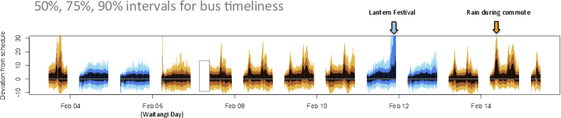
    It is better if
    all actions that make up a final plot can be
    captured in code and therefore recorded, automated, and shared.
    In this particular context, the variable-width line facility
    is meant to obviate the need for something like Adobe Illustrator's 
    <a href="ttps://helpx.adobe.com/illustrator/atv/cs5-tutorials/using-variablewidth-strokes.html">variable-width stroke tool</a>,
    or SynFig's 
    <a href="http://wiki.synfig.org/Advanced_Outline_Layer">Advanced Outline
    Layer</a>.   
    This work is also influenced by 
    the 
    <a href="https://www.w3.org/Graphics/SVG/WG/wiki/Proposals/Variable_width_stroke">SVG proposal for variable-width lines</a> (also see the discussion by
    <a href="http://www.schepers.cc/differentstrokes.html">Doug Schepers</a>)
    and the 
    <a href="http://wiki.inkscape.org/wiki/index.php/PowerStroke">Inkscape
    power stroke proposal</a>.
  </p>
    <h2>
      <a name="method-1">Method 1: Offsetting points</a>
    </h2>
    <p>
    The first approach to drawing a variable-width line with 'vwline'
    is provided by the <code>grid.vwcurve</code> function.  This function
    accepts a set of x/y locations and a set of widths, all of which 
    recycle as necessary.  The idea with this function is that we know 
    the placement of the line and the
    width of the line at all points on a curve.  
  </p>
    <p>
    The function generates (and draws) a polygon using the following 
    algorithm:
  </p>
    <ol type="A">
      <li>
      The centre of the line is specified by x/y locations; the line
      is a series of straight line segments.
    </li>
      <li>
      A perpendicular is calculated at each point on the line; the angle
      of the perpendicular is based on the slopes of the line segments
      either side of the point (or just the following/preceding line
      segment at the start/end of the line).
    </li>
      <li>
      A "left" border is generated by connecting all left ends of the
      perpendiculars (where left is defined as if we are moving along
      the line in the order of the x/y locations).  Similar for the
      "right" border.
    </li>
      <li>
      A polygon is generated by combining the left border with the reversed
      right border.
    </li>
    </ol>
    <rcode echo="FALSE"><![CDATA[
vwcurvediagram <- function(step) {
    x <- c(.2, .6, .8)
    y <- c(.8, .6, .2)
    w <- c(.05, .1, .2)
    vwgrob <- vwcurveGrob(x, y, w)
    sub <- function() {
        ## Points on line
        grid.points(x, y, pch=16, gp=gpar(col="black"))
        grid.lines(x, y)
        if (step < 2) return()
        grid.rect(width=.92, height=.92, gp=gpar(col=NA, fill=rgb(1,1,1,.8)))
        pts <- vwline:::vwcurvePoints(vwgrob)
        grid.segments(pts$left$x, pts$left$y, pts$right$x, pts$right$y,
                      default.units="in")
        if (step < 3) return()
        grid.rect(width=.92, height=.92, gp=gpar(col=NA, fill=rgb(1,1,1,.8)))
        grid.segments(pts$left$x[-3], pts$left$y[-3], 
                      pts$left$x[-1], pts$left$y[-1],
                      default.units="in",
                      arrow=arrow(angle=20, length=unit(3, "mm"),
                                  type="closed"),
                      gp=gpar(col="blue", fill="blue"))
        grid.segments(pts$right$x[-3], pts$right$y[-3], 
                      pts$right$x[-1], pts$right$y[-1],
                      default.units="in",
                      arrow=arrow(angle=20, length=unit(3, "mm"),
                                  type="closed"),
                      gp=gpar(col="red", fill="red"))
        if (step < 4) return()
        grid.rect(width=.92, height=.92, gp=gpar(col=NA, fill=rgb(1,1,1,.8)))
        grid.segments(c(pts$left$x, rev(pts$right$x)),
                      c(pts$left$y, rev(pts$right$y)),
                      c(pts$left$x[-1], rev(pts$right$x), pts$left$x[1]),
                      c(pts$left$y[-1], rev(pts$right$y), pts$left$y[1]),
                      default.units="in",
                      arrow=arrow(angle=20, length=unit(3, "mm"),
                                  type="closed"))
    }
    grid.newpage()
    pushViewport(viewport(gp=gpar(lwd=3)))
    sub()
    grid.rect(width=.95, height=.95)
    grid.text(LETTERS[step], .15, .15, gp=gpar(cex=4))
}
  ]]></rcode>
    <rcode results="hide" echo="FALSE"><![CDATA[
for (i in 1:4) {
    svg(paste0("figure/vwcurvediag-", i, ".svg"), width=5, height=5, bg="transparent")  
    vwcurvediagram(i)
    dev.off()
}
  ]]></rcode>
    <img src="figure/vwcurvediag-1.svg" width="30%"/>
    <img src="figure/vwcurvediag-2.svg" width="30%"/>
    <img src="figure/vwcurvediag-3.svg" width="30%"/>
    <img src="figure/vwcurvediag-4.svg" width="30%"/>
    <p>
    This function
    can be used to produce the sort of result that 'beanplot' and other packages
    already provide, but with the additional flexibility that the
    line does not have to be straight and the widths do not have to be
    aligned with the x-axis or with the y-axis.  In the images below,
    the main variable-width line is thick and black; a thin white line is drawn
    to represent the x/y locations of the centre of the line.
  </p>
    <rcode><![CDATA[
library(vwline)
  ]]></rcode>
    <rcode id="vwcurve" echo="3:6" dev="mysvg" fig.width="3" fig.height="3" fig.ext="svg" fig.show="hide"><![CDATA[
grid.rect(gp=gpar(col=NA, fill="grey90"))
pushViewport(viewport(width=.8, height=.8))
d <- density(ToothGrowth$len)
x <- (d$x - min(d$x))/diff(range(d$x))
w <- .2*d$y/max(d$y)
grid.vwcurve(x, .5, w)
grid.lines(x, .5, gp=gpar(col="white", lwd=1))
grid.text("vwcurve()", y=.1, gp=gpar(fontfamily="mono"))
  ]]></rcode>
    <rcode id="vwcurve-curve" echo="3:6" dev="mysvg" fig.width="3" fig.height="3" fig.ext="svg" fig.show="hide"><![CDATA[
grid.rect(gp=gpar(col=NA, fill="grey90"))
pushViewport(viewport(width=.8, height=.8))
t <- seq(0, 2*pi, length.out=length(d$x))
x <- .5 + .3*cos(t)
y <- .5 + .3*sin(t)
grid.vwcurve(x, y, w)
grid.lines(x, y, gp=gpar(col="white", lwd=1))
grid.text("vwcurve()", y=.1, gp=gpar(fontfamily="mono"))
  ]]></rcode>
    <p class="img">
      <img src="figure/vwcurve-1.svg" width="30%"/>
      <img src="figure/vwcurve-curve-1.svg" width="30%"/>
    </p>
    <h2>
      <a name="method-2">Method 2: Offsetting control points</a>
    </h2>
    <p>
    The second approach to drawing variable-width lines, which is provided
    by the <code>grid.vwXspline</code> function, also accepts
    x/y locations, plus a set of widths, but this time the 
    locations describe control points for a curve, rather than
    explicit locations for the line to pass through.  
  </p>
    <p>
    More specifically, with this approach
    the x/y locations describe the control points for an X-spline, and
    the widths describe an amount to offset additional control points
    to the left and right of the main control points.
    The algorithm used to generate a polygon is as follows:
  </p>
    <ol type="A">
      <li>
      The centre of the line is specified by x/y control points; the line
      approximates the control points.
    </li>
      <li>
      A perpendicular is calculated at each control point - the angle
      of the perpendicular is based on the slopes of the line segments
      connecting neighbouring control points - and a new control point is
      added at each end of the perpendicular.
    </li>
      <li>
      A "left" border is generated as an X-spline based on the left 
      control points (where left is defined as if we are moving between
      the control points in the order of the x/y locations).  Similar for the
      "right" border.
    </li>
      <li>
      A polygon is generated by combining the left border with the reversed
      right border.
    </li>
    </ol>
    <p>
    This approach is similar to work on simulating brush strokes by 
    <a href="#pham">Pham</a> and, to a lesser extent,
    <a href="#chua">Chua</a>.  
    <a href="#klassen">Klassen</a> also discusses this sort of
    approach for representing fonts.  
  </p>
    <rcode echo="FALSE"><![CDATA[
vwxsplinediagram <- function(step) {
    x <- c(.2, .6, .8)
    y <- c(.8, .6, .2)
    w <- c(.05, .1, .2)
    sub <- function() {
        ## Control points
        grid.points(x, y, pch=16, gp=gpar(col="black"))
        ## Xspline 
        grid.xspline(x, y, shape=1)
        if (step < 2) return()
        grid.rect(width=.92, height=.92, gp=gpar(col=NA, fill=rgb(1,1,1,.8)))
        vwgrob <- vwcurveGrob(x, y, w)
        pts <- vwline:::vwcurvePoints(vwgrob)
        grid.segments(pts$left$x, pts$left$y, pts$right$x, pts$right$y,
                      default.units="in")
        if (step < 3) return()
        grid.rect(width=.92, height=.92, gp=gpar(col=NA, fill=rgb(1,1,1,.8)))
        grid.points(pts$left$x, pts$left$y, default.units="in",
                    pch=16, gp=gpar(col="blue"))
        grid.xspline(pts$left$x, pts$left$y, default.units="in", shape=1,
                     gp=gpar(col="blue"),
                     arrow=arrow(angle=20, length=unit(3, "mm"),
                                  type="closed"))
        grid.points(pts$right$x, pts$right$y, default.units="in",
                    pch=16, gp=gpar(col="red"))
        grid.xspline(pts$right$x, pts$right$y, default.units="in", shape=1,
                     gp=gpar(col="red"), 
                     arrow=arrow(angle=20, length=unit(3, "mm"),
                                 type="closed"))
        if (step < 4) return()
        grid.rect(width=.92, height=.92, gp=gpar(col=NA, fill=rgb(1,1,1,.8)))
        leftPts <- xsplinePoints(xsplineGrob(pts$left$x, pts$left$y, 
                                             default.units="in", shape=1))
        rightPts <- xsplinePoints(xsplineGrob(pts$right$x, pts$right$y, 
                                              default.units="in", shape=1))
        grid.xspline(pts$left$x, pts$left$y, default.units="in", shape=1,
                     gp=gpar(fill="black"),
                     arrow=arrow(angle=20, length=unit(3, "mm"),
                                  type="closed"))
        grid.xspline(rev(pts$right$x), rev(pts$right$y),
                     default.units="in", shape=1,
                     gp=gpar(fill="black"),
                     arrow=arrow(angle=20, length=unit(3, "mm"),
                                  type="closed"))
        grid.segments(leftPts$x[length(leftPts$x)], 
                      leftPts$y[length(leftPts$x)], 
                      rightPts$x[length(rightPts$x)],
                      rightPts$y[length(rightPts$x)],
                      default.units="in",
                      arrow=arrow(angle=20, length=unit(3, "mm"),
                                  type="closed"))
        grid.segments(rightPts$x[1],
                      rightPts$y[1],
                      leftPts$x[1], 
                      leftPts$y[1], 
                      default.units="in",
                      arrow=arrow(angle=20, length=unit(3, "mm"),
                                  type="closed"))
    }
    grid.newpage()
    pushViewport(viewport(gp=gpar(lwd=3)))
    sub()
    grid.rect(width=.95, height=.95)
    grid.text(LETTERS[step], .15, .15, gp=gpar(cex=4))
}
  ]]></rcode>
    <rcode results="hide" echo="FALSE"><![CDATA[
for (i in 1:4) {
    svg(paste0("figure/vwxsplinediag-", i, ".svg"), width=5, height=5, bg="transparent")  
    vwxsplinediagram(i)
    dev.off()
}
  ]]></rcode>
    <img src="figure/vwxsplinediag-1.svg" width="30%"/>
    <img src="figure/vwxsplinediag-2.svg" width="30%"/>
    <img src="figure/vwxsplinediag-3.svg" width="30%"/>
    <img src="figure/vwxsplinediag-4.svg" width="30%"/>
    <p>
    This function can be useful if we want to produce a variable-width 
    curve, but do not want to specify every x/y location and width
    for the curve.  In other words, we want to draw a smooth curve
    with smoothly-varying width, without having to specify the curve or
    the width in minute detail.
  </p>
    <rcode id="vwxspline-curve" echo="3:6" dev="mysvg" fig.width="3" fig.height="3" fig.ext="svg" fig.show="hide"><![CDATA[
grid.rect(gp=gpar(col=NA, fill="grey90"))
pushViewport(viewport(width=.8, height=.8))
x <- c(0, .5, 1)
y <- c(.5, .5, .5)
w <- c(0, .2, 0)
grid.vwXspline(x, y, w, shape=-1)
grid.xspline(x, y, shape=-1, gp=gpar(col="white", lwd=1))
grid.text("vwXspline()", y=.1, gp=gpar(fontfamily="mono"))
  ]]></rcode>
    <rcode id="vwxspline-swish" echo="3:6" dev="mysvg" fig.width="3" fig.height="3" fig.ext="svg" fig.show="hide"><![CDATA[
grid.rect(gp=gpar(col=NA, fill="grey90"))
pushViewport(viewport(width=.8, height=.8))
x <- 0:3/3
y <- c(.5, .7, .3, .5)
w <- c(0, .2, .2, 0)
grid.vwXspline(x, y, w)
grid.xspline(x, y, shape=1, gp=gpar(col="white", lwd=1))
grid.text("vwXspline()", y=.1, gp=gpar(fontfamily="mono"))
  ]]></rcode>
    <p class="img">
      <img src="figure/vwxspline-curve-1.svg" width="30%"/>
      <img src="figure/vwxspline-swish-1.svg" width="30%"/>
    </p>
    <h2>
      <a name="method-3">Method 3: Offsetting line segments</a>
    </h2>
    <p>
    The third approach to drawing variable-width lines is
    provided by the <code>vwline</code> function.  This is similar
    to the <code>vwcurve</code> function, because every location
    and width for the line is specified explicitly, but it is
    designed for a situation where the main line really is a series
    of straight line segments (e.g., Minard's map).
    The difference is that this function treats each location 
    as a corner (where <code>vwcurve</code> pretends that the line is 
    a smooth curve with no sharp corners).
  </p>
    <ol type="A">
      <li>
      The centre of the line is specified by x/y locations; the line
      is a series of straight line segments.
    </li>
      <li>
      A perpendicular is calculated at both ends of every line segment,
      using the specified width value for each location.  This produces
      a series of thick segments.
    </li>
      <li>
      A "left" border is generated by traversing the left edge of each thick 
      line segment (where left is defined as if we are moving along
      the line in the order of the x/y locations).  Gaps at the outsides of
      corners are spanned using a linejoin style (see
      <a href="#linejoins">Line joins</a>).  The insides of corners are
      resolved by joining the end of the edge of segment <i>i</i> with the 
      corner location then with the start of the edge of segment
      <i>i + 1</i>. Similar for the "right" border.
    </li>
      <li>
      A polygon is generated by combining the left border with the reversed
      right border and simplifying the resulting polygon 
      (using <code>polysimplify</code> from the 'polyclip' package).
    </li>
    </ol>
    <rcode echo="FALSE"><![CDATA[
vwlinediagram <- function(step) {
    x <- c(.2, .6, .8)
    y <- c(.8, .6, .2)
    w <- c(.05, .1, .2)
    vwgrob <- vwlineGrob(x, y, w)
    sub <- function() {
        ## Points on line
        grid.points(x, y, pch=16, gp=gpar(col="black"))
        grid.lines(x, y)
        if (step < 2) return()

        grid.rect(width=.92, height=.92, gp=gpar(col=NA, fill=rgb(1,1,1,.8)))
        xx <- convertX(unit(x, "npc"), "in", valueOnly=TRUE)
        yy <- convertY(unit(y, "npc"), "in", valueOnly=TRUE)
        ww <- pmin(convertWidth(unit(w, "npc"), "in", valueOnly=TRUE),
                   convertHeight(unit(w, "npc"), "in", valueOnly=TRUE))
        ww <- list(left=ww/2, right=ww/2)
        sinfo <- vwline:::segInfo(xx, yy, ww, TRUE, FALSE, FALSE)
        with(sinfo,
             grid.polygon(c(perpStartLeftX, perpEndLeftX,
                            perpEndRightX, perpStartRightX),
                          c(perpStartLeftY, perpEndLeftY,
                            perpEndRightY, perpStartRightY),
                          default.units="in",
                          id=rep(1:(length(xx) - 1), 4))
             )
        if (step < 3) return()

        grid.rect(width=.92, height=.92, gp=gpar(col=NA, fill=rgb(1,1,1,.8)))
        pts <- vwline:::vwlinePoints(vwlineGrob(x, y, w))
        grid.lines(pts$left$x, pts$left$y, default.units="in",
                   gp=gpar(col="blue"))
        grid.lines(pts$right$x, pts$right$y, default.units="in",
                   gp=gpar(col="red"))
        if (step < 4) return()

        grid.rect(width=.92, height=.92, gp=gpar(col=NA, fill=rgb(1,1,1,.8)))
        o <- vwline:::vwlineOutline(vwlineGrob(x, y, w, lineend="butt"))[[1]]
        grid.polygon(o$x, o$y, default.units="in")
    }
    grid.newpage()
    pushViewport(viewport(gp=gpar(lwd=3)))
    sub()
    grid.rect(width=.95, height=.95)
    grid.text(LETTERS[step], .15, .15, gp=gpar(cex=4))
}
  ]]></rcode>
    <rcode results="hide" echo="FALSE"><![CDATA[
for (i in 1:4) {
    svg(paste0("figure/vwlinediag-", i, ".svg"), width=5, height=5, bg="transparent")  
    vwlinediagram(i)
    dev.off()
}
  ]]></rcode>
    <img src="figure/vwlinediag-1.svg" width="30%"/>
    <img src="figure/vwlinediag-2.svg" width="30%"/>
    <img src="figure/vwlinediag-3.svg" width="30%"/>
    <img src="figure/vwlinediag-4.svg" width="30%"/>
    <p>
    This function produces a non-smooth line, which may be useful
    if we wish to emphasise that the width is only known at specific
    locations along the line.
  </p>
    <rcode id="vwline-swish" echo="3:6" dev="mysvg" fig.width="3" fig.height="3" fig.ext="svg" fig.show="hide"><![CDATA[
grid.rect(gp=gpar(col=NA, fill="grey90"))
pushViewport(viewport(width=.8, height=.8))
x <- 0:3/3
y <- c(.5, .7, .3, .5)
w <- c(0, .2, .2, 0)
grid.vwline(x, y, w)
grid.lines(x, y, gp=gpar(col="white", lwd=1))
grid.text("vwline()", y=.1, gp=gpar(fontfamily="mono"))
  ]]></rcode>
    <p class="img">
      <img src="figure/vwline-swish-1.svg" width="30%"/>
    </p>
    <h2>
      <a name="method-4">Method 4: Sweeping curves with a brush</a>
    </h2>
    <p>
    The fourth approach to drawing variable-width lines, which is
    provided by the <code>brushXspline</code> function, takes
    a set of x/y control points to describe the line (an X-spline), a
    "brush" (a geometric shape) 
    that is used to "sweep" the line, plus a set of widths
    that are used to scale the brush as it moves along the line.
  </p>
    <ol type="A">
      <li>
      The centre of the line is specified by x/y control points;
      the line approximates the control points.
    </li>
      <li>
      The centre of the line is "flattened" to a series of 
      short straight line segments.
    </li>
      <li>
      The brush is placed at each vertex on the flattened line,
      with the brush angled perpendicular to the flattened line 
      and the brush is scaled based on the width of the line at each vertex.
    </li>
      <li>
      A shape is generated from the convex hull of the first pair
      pair of brushes.
    </li>
      <li>
      This is repeated for each consecutive pair of brushes.
    </li>
      <li>
      A polygon is generated by combining 
      the convex hulls using a union operation.
    </li>
    </ol>
    <p>
    This approach 
    is not entirely unlike <a href="metafont">Knuth's MetaFont</a>,
    though with far less control over the path that is to be swept.
  </p>
    <rcode echo="FALSE"><![CDATA[
diagram <- function(step) {
    x <- c(.2, .6, .8)
    y <- c(.8, .6, .2)
    w <- c(.3, .5, .7)
    sub <- function() {
        ## Control points
        grid.points(x, y, pch=16, gp=gpar(col="black"))
        ## Xspline 
        grid.xspline(x, y, shape=1)
        if (step < 2) return()
        grid.rect(width=.92, height=.92, gp=gpar(col=NA, fill=rgb(1,1,1,.8)))
        pts <- xsplinePoints(xsplineGrob(x, y, shape=1))
        n <- length(pts$x)
        pts <- list(x=c(pts$x[1], pts$x[n %/% 2], pts$x[n]),
                    y=c(pts$y[1], pts$y[n %/% 2], pts$y[n]))
        grid.lines(pts$x, pts$y, "in")
        if (step < 3) return()
        grid.rect(width=.92, height=.92, gp=gpar(col=NA, fill=rgb(1,1,1,.8)))
        brushes <- list(vwline:::placeBrush(verticalBrush, pts$x[1], pts$y[1], w[1],
                                   vwline:::angle(pts$x[1:2], pts$y[1:2])),
                        vwline:::placeBrush(verticalBrush, pts$x[2], pts$y[2], w[2],
                                   (vwline:::angle(pts$x[1:2], pts$y[1:2]) + 
                                   vwline:::angle(pts$x[2:3], pts$y[2:3]))/2),
                        vwline:::placeBrush(verticalBrush, pts$x[3], pts$y[3], w[3],
                                   vwline:::angle(pts$x[2:3], pts$y[2:3])))
        lapply(brushes, function(x) grid.polygon(x$x, x$y, default.units="in"))
        if (step < 4) return()
        grid.rect(width=.92, height=.92, gp=gpar(col=NA, fill=rgb(1,1,1,.8)))
        seg1 <- list(x=c(brushes[[1]]$x, brushes[[2]]$x), 
                     y=c(brushes[[1]]$y, brushes[[2]]$y))
        h1 <- chull(seg1)
        grid.polygon(seg1$x[h1], seg1$y[h1], default.units="in")
        if (step < 5) return()
        seg2 <- list(x=c(brushes[[2]]$x, brushes[[3]]$x), 
                     y=c(brushes[[2]]$y, brushes[[3]]$y))
        h2 <- chull(seg2)
        grid.polygon(seg2$x[h2], seg2$y[h2], default.units="in")
        if (step < 6) return()
        grid.rect(width=.92, height=.92, gp=gpar(col=NA, fill=rgb(1,1,1,.8)))
        final <- Reduce(vwline:::combineShapes, 
                        list(list(x=seg1$x[h1], y=seg1$y[h1]),
                             list(x=seg2$x[h2], y=seg2$y[h2])))[[1]]
        grid.polygon(final$x, final$y, default.units="in")    
    }
    grid.newpage()
    pushViewport(viewport(gp=gpar(lwd=3)))
    sub()
    grid.rect(width=.95, height=.95)
    grid.text(LETTERS[step], .15, .15, gp=gpar(cex=4))
}
  ]]></rcode>
    <rcode results="hide" echo="FALSE"><![CDATA[
for (i in 1:6) {
    svg(paste0("figure/diag-", i, ".svg"), width=5, height=5, bg="transparent")  
    diagram(i)
    dev.off()
}
  ]]></rcode>
    <img src="figure/diag-1.svg" width="30%"/>
    <img src="figure/diag-2.svg" width="30%"/>
    <img src="figure/diag-3.svg" width="30%"/>
    <img src="figure/diag-4.svg" width="30%"/>
    <img src="figure/diag-5.svg" width="30%"/>
    <img src="figure/diag-6.svg" width="30%"/>
    <p>
    The <code>brushXspline</code>
    function can be useful if we want to produce a variable-width 
    curve and do not want to specify every x/y location or width
    for the curve (so cannot use <code>vwcurve</code> or 
    <code>vwline</code>), 
    but we want the perpendicular width of the curve
    to be more accurately represented (so cannot use <code>vwXspline</code>).
  </p>
    <p>
    The examples below construct a <code>vwXspline</code> and a 
    <code>brushXspline</code> through the same set of control points.
    In the <code>brushXspline</code> case, we can see the effect
    of the width being perpendicular to the line at all points along the line.
  </p>
    <rcode id="vwxspline-swish-text" echo="3:6" dev="mysvg" fig.width="3" fig.height="3" fig.ext="svg" fig.show="hide"><![CDATA[
grid.rect(gp=gpar(col=NA, fill="grey90"))
pushViewport(viewport(width=.8, height=.8))
x <- 0:3/3
y <- c(.5, .7, .3, .5)
w <- c(0, .2, .2, 0)
grid.vwXspline(x, y, w)
grid.xspline(x, y, shape=1, gp=gpar(col="white", lwd=1))
grid.text("vwXspline()", y=.1, gp=gpar(fontfamily="mono"))
  ]]></rcode>
    <rcode id="brushxspline-swish" echo="3:6" dev="mysvg" fig.width="3" fig.height="3" fig.ext="svg" fig.show="hide"><![CDATA[
grid.rect(gp=gpar(col=NA, fill="grey90"))
pushViewport(viewport(width=.8, height=.8))
x <- 0:3/3
y <- c(.5, .7, .3, .5)
w <- c(0, .2, 0)
grid.brushXspline(verticalBrush, x, y, w)
grid.xspline(x, y, shape=1, gp=gpar(col="white", lwd=1))
grid.text("brushXspline()", y=.1, gp=gpar(fontfamily="mono"))
  ]]></rcode>
    <p class="img">
      <img src="figure/vwxspline-swish-text-1.svg" width="30%"/>
      <img src="figure/brushxspline-swish-1.svg" width="30%"/>
    </p>
    <h2>
      <a name="method-4">Method 5: Offsetting curves</a>
    </h2>
    <p>
    The final approach, provided by the <code>offsetXspline</code> function,
    generates a mathematical description of
    "offset curves" and draws those offset curves.
  </p>
    <p>
    The problem of determining the outline for a curve, when the 
    width is fixed, is known as generating an "offset curve" or
    an "offset polygon".
    This arises in a variety of contexts, including stroking a
    path with a non-zero line width, and producing buffer regions
    for spatial objects.
    With offset curves, we start with a 
    mathematical definition of the curve (e.g., a Bezier curve),
    and we derive a mathematical expression for curves that are offset by
    a fixed amount, then we render the offset curve.
  </p>
    <p>
    Examples of mathematical 
    solutions for offset curves are often focused on
    Bezier curves, e.g., <a href="#hoschek">Hoschek</a> and
    <a href="#hain">Hain et al</a>.  A review was given by 
    <a href="#elber">Elber et al</a>.
  </p>
    <p>
    A general approach for offset polygons was described by 
    <a href="#polygon-offsetting">Chen and McMains</a>.
    This algorithm has been implemented in the 
    <a href="#clipper">Clipper</a> library, which has an R interface via
    the <a href="#polyclip">polyclip</a> package.
    The <a href="http://www.cgal.org/">CGAL</a> 
    library can also generate polygon
    offsets, particularly the 
    <a href="#cgal-polygon-offset-manual">2D Straight Skeleton and Polygon Offsetting</a>
    package.
  </p>
    <p>
    This function implements the general formulation for a variable
    offset curve that is described in <a href="#chen+lin">Chen and Lin</a>.
    The difficult part of this approach is determining a function for the 
    offset curve (which requires a function for the unit normal to the main 
    curve and a function for the width of the curve).
    However, once these equations have been found,
    the algorithm is straightforward.
  </p>
    <ol type="A">
      <li>
      The centre of the line is specified by x/y control points;
      the line approximates the control points.
    </li>
      <li>
      The centre of the line is "flattened" to a series of 
      short straight line segments.
    </li>
      <li>
      Perpendiculars are found by evaluating the 
      unit normal and the line width at
      each vertex (the end of the perpendicular
      is the vertex plus the unit normal
      multiplied by the width).  
    </li>
      <li>
      A "left" border is generated by connecting all left ends of the
      perpendiculars (where left is defined as if we are moving along
      the line in the order of the x/y locations).  Similar for the
      "right" border.      
    </li>
      <li>
      A polygon is generated by combining the left border with the reversed
      right border and simplifying the resulting polygon 
      (using <code>polysimplify</code> from the 'polyclip' package).
    </li>
    </ol>
    <rcode echo="FALSE"><![CDATA[
offsetxsplinediagram <- function(step) {
    x <- c(.2, .6, .8)
    y <- c(.8, .6, .2)
    w <- c(.05, .1, .2)
    vwgrob <- offsetXsplineGrob(x, y, w)
    sub <- function() {
        ## Control points
        grid.points(x, y, pch=16, gp=gpar(col="black"))
        ## Xspline 
        grid.xspline(x, y, shape=1)
        if (step < 2) return()

        grid.rect(width=.92, height=.92, gp=gpar(col=NA, fill=rgb(1,1,1,.8)))
        pts <- vwline:::offsetXsplinePoints(vwgrob)
        n <- length(pts$mid$x)
        pts <- lapply(pts, 
                      function(x) { 
                          subset <- c(1, (1:n)[(1:n) %% 3 == 0], n)
                          list(x=c(x$x[subset]),
                               y=c(x$y[subset])) 
                      })
        grid.lines(pts$mid$x, pts$mid$y, "in")
        if (step < 3) return()

        grid.rect(width=.92, height=.92, gp=gpar(col=NA, fill=rgb(1,1,1,.8)))
        grid.segments(pts$mid$x, pts$mid$y, pts$left$x, pts$left$y, 
                      default.units="in", gp=gpar(col="blue"))
        grid.segments(pts$mid$x, pts$mid$y, pts$right$x, pts$right$y, 
                      default.units="in", gp=gpar(col="red"))
        if (step < 4) return()

        grid.rect(width=.92, height=.92, gp=gpar(col=NA, fill=rgb(1,1,1,.8)))
        pts <- vwline:::offsetXsplinePoints(vwgrob)
        grid.lines(pts$left$x, pts$left$y, default.units="in",
                   gp=gpar(col="blue"))
        grid.lines(pts$right$x, pts$right$y, default.units="in",
                   gp=gpar(col="red"))
        if (step < 5) return()

        grid.rect(width=.92, height=.92, gp=gpar(col=NA, fill=rgb(1,1,1,.8)))
        o <- vwline:::offsetXsplineOutline(vwgrob)[[1]]
        grid.polygon(o$x, o$y, default.units="in")
    }
    grid.newpage()
    pushViewport(viewport(gp=gpar(lwd=3)))
    sub()
    grid.rect(width=.95, height=.95)
    grid.text(LETTERS[step], .15, .15, gp=gpar(cex=4))
}
  ]]></rcode>
    <rcode results="hide" echo="FALSE"><![CDATA[
for (i in 1:5) {
    svg(paste0("figure/offsetxsplinediag-", i, ".svg"), width=5, height=5, bg="transparent")  
    offsetxsplinediagram(i)
    dev.off()
}
  ]]></rcode>
    <img src="figure/offsetxsplinediag-1.svg" width="30%"/>
    <img src="figure/offsetxsplinediag-2.svg" width="30%"/>
    <img src="figure/offsetxsplinediag-3.svg" width="30%"/>
    <img src="figure/offsetxsplinediag-4.svg" width="30%"/>
    <img src="figure/offsetxsplinediag-5.svg" width="30%"/>
    <p>
    The result from this function should be similar to the 
    result from <code>brushXspline</code> (as shown below).
    The <code>offsetXspline</code> function provides a more robust (less
    heuristic) approach, but <code>brushXspline</code> offers more
    flexibility via the possibility of different brushes
    (see <a href="#brushes">Specifying brushes</a>).
  </p>
    <rcode id="offsetxspline-swish" echo="3:6" dev="mysvg" fig.width="3" fig.height="3" fig.ext="svg" fig.show="hide"><![CDATA[
grid.rect(gp=gpar(col=NA, fill="grey90"))
pushViewport(viewport(width=.8, height=.8))
x <- 0:3/3
y <- c(.5, .7, .3, .5)
w <- c(0, .2, 0)
grid.offsetXspline(x, y, w)
grid.xspline(x, y, shape=1, gp=gpar(col="white", lwd=1))
grid.text("offsetXspline()", y=.1, gp=gpar(fontfamily="mono"))
  ]]></rcode>
    <p class="img">
      <img src="figure/brushxspline-swish-1.svg" width="30%"/>
      <img src="figure/offsetxspline-swish-1.svg" width="30%"/>
    </p>
    <h2>
      <a name="Detail">Fine tuning variable-width lines</a>
    </h2>
    <p>
    Having introduced the basic idea behind the main functions
    in the 'vwline' package, we will now explore how these functions
    work in a little more detail.
  </p>
    <h3>
      <a name="line-width">Specifying line width</a>
    </h3>
    <p>
    For the functions <code>vwcurve</code>, <code>vwline</code>,
    and <code>vwXspline</code>,
    we specify widths explicitly, 
    either as a width for 
    every x/y location on the line or as
    a width for every x/y control point.
  </p>
    <p>
    For <code>vwcurve</code>
    and <code>vwXspline</code>,
    widths are just a numeric vector or a 'grid' unit and
    the width is the same either side of the main curve.
    The <code>vwline</code> function is slightly more flexible and
    accepts a numeric vector or
    'grid' unit for the width, but also accepts a list of separate
    left and right widths, as generated by the <code>widthSpec</code>
    function.  This allows different widths to the left and right
    of the main curve.
  </p>
    <rcode id="width-numeric" echo="3:5" dev="mysvg" fig.width="3" fig.height="3" fig.ext="svg" fig.show="hide"><![CDATA[
grid.rect(gp=gpar(col=NA, fill="grey90"))
pushViewport(viewport(width=.8, height=.8))
x <- 0:1
y <- c(.5, .5)
grid.vwline(x, y, w=c(.1, .2))
grid.lines(x, y, gp=gpar(col="white"))
grid.text("numeric width", y=.1, gp=gpar(fontfamily="mono"))
  ]]></rcode>
    <rcode id="width-unit" echo="3" dev="mysvg" fig.width="3" fig.height="3" fig.ext="svg" fig.show="hide"><![CDATA[
grid.rect(gp=gpar(col=NA, fill="grey90"))
pushViewport(viewport(width=.8, height=.8))
grid.vwline(x, y, w=unit(1:2, "cm"))
grid.lines(x, y, gp=gpar(col="white"))
grid.text("unit width", y=.1, gp=gpar(fontfamily="mono"))
  ]]></rcode>
    <rcode id="width-spec" echo="3" dev="mysvg" fig.width="3" fig.height="3" fig.ext="svg" fig.show="hide"><![CDATA[
grid.rect(gp=gpar(col=NA, fill="grey90"))
pushViewport(viewport(width=.8, height=.8))
grid.vwline(x, y, w=widthSpec(list(left=c(.1, .2), right=unit(2:1, "cm"))))
grid.lines(x, y, gp=gpar(col="white"))
grid.text("widthSpec()", y=.1, gp=gpar(fontfamily="mono"))
  ]]></rcode>
    <p class="img">
      <img src="figure/width-numeric-1.svg" width="30%"/>
      <img src="figure/width-unit-1.svg" width="30%"/>
      <img src="figure/width-spec-1.svg" width="30%"/>
    </p>
    <!--
  <p>
    Use data/alaska-anchorage.txt temperature data to demonstrate
    separate leftWidth and rightWidth in widthSpec().
  </p>
-->
    <p>
    The <code>vwline</code> function also has a <code>stepWidth</code>
    argument, which means that widths are not linearly interpolated along
    the main curve, but remain constant along each segment (and the final
    width is silently ignored).
  </p>
    <rcode id="width-interp" echo="3:6" dev="mysvg" fig.width="3" fig.height="3" fig.ext="svg" fig.show="hide"><![CDATA[
grid.rect(gp=gpar(col=NA, fill="grey90"))
pushViewport(viewport(width=.8, height=.8))
x <- 0:3/3
y <- c(.4, .6, .4, .6)
w <- c(.1, .2, .3, .2)
grid.vwline(x, y, w)
grid.lines(x, y, gp=gpar(col="white"))
grid.text("stepWidth=FALSE", y=.1, gp=gpar(fontfamily="mono"))
  ]]></rcode>
    <rcode id="width-step" echo="3" dev="mysvg" fig.width="3" fig.height="3" fig.ext="svg" fig.show="hide"><![CDATA[
grid.rect(gp=gpar(col=NA, fill="grey90"))
pushViewport(viewport(width=.8, height=.8))
grid.vwline(x, y, w, stepWidth=TRUE)
grid.lines(x, y, gp=gpar(col="white"))
grid.text("stepWidth=TRUE", y=.1, gp=gpar(fontfamily="mono"))
  ]]></rcode>
    <p class="img">
      <img src="figure/width-interp-1.svg" width="30%"/>
      <img src="figure/width-step-1.svg" width="30%"/>
    </p>
    <p>
    For the <code>brushXspline</code> and <code>offsetXspline</code> functions, 
    the line width
    is not as tightly coupled with the x/y locations.
    For these functions, the x/y locations describe a curve
    and the width argument separately describes how the line width
    should vary along the length of the curve.  The simplest approach
    is to specify a numeric vector of width values, in which case the 
    first value is used as the width at the start of the curve, the last 
    value is used as the width at the end of the curve, and the other
    widths are spaced evenly along the curve.  By default, the
    widths are interpreted as numbers of millimetres.
  </p>
    <p>
    By default, 
    the change in width along the line is controlled by an X-spline
    with a shape parameter of -1.  The
    <code>brushXspline</code> example from the previous section is
    repeated below (the left image).  
    Notice that there are four x/y locations for
    control points, but only three width values.  This means that
    the width of the line starts at 0, ends at 0, and is 0.2 in the
    middle of the curve, with width varying smoothly according to an X-spline
    through (0, 0), (0.5, 0.2), (1, 0).  The image below on the right 
    shows what this width X-spline looks like.
  </p>
    <rcode eval="FALSE" ref.label="brushxspline-swish" echo="3:6"><![CDATA[
  ]]></rcode>
    <rcode id="width-spline" echo="FALSE" dev="mysvg" fig.width="3" fig.height="3" fig.ext="svg" fig.show="hide"><![CDATA[
grid.rect(gp=gpar(col=NA, fill="grey90"))
pushViewport(viewport(width=.8, height=.8))
x <- c(0, .5, 1)
y <- c(.5, .7, .5) - .1
grid.lines(c(0, 0, 1), c(1, 0.5, 0.5) - .1, gp=gpar(col="white"))
grid.xspline(x, y, shape=-1)
grid.text("line width", x=unit(-1, "line"), y=.6, rot=90)
grid.text("distance along curve", y=.3)
  ]]></rcode>
    <p class="img">
      <img src="figure/brushxspline-swish-1.svg" width="30%"/>
      <img src="figure/width-spline-1.svg" width="30%"/>
    </p>
    <p>
    The spline that controls the width for <code>brushXspline</code> 
    and <code>offsetXspline</code> can also be 
    specified explicitly with the <code>widthSpline</code> function.
    This allows the set of widths to be defined along with a set of distances
    along the line (the x-values for the width X-spline).  
    The distances can just
    be numeric values, in which case they are interpreted as proportions
    of the line length, or they can be 'grid' units (e.g., millimetres).
    There is also a <code>shape</code> argument to control the shape of the 
    width X-spline (though note that positive shape values
    will mean that the maximum explicit width may not be achieved; see
    <a href="#xsplines">the appendix on X-splines</a>).  Finally, there
    is a <code>rep</code> argument to control whether the widths
    repeat or stay fixed for distances along the curve that are outside
    the explicit distances specified by the width spline.
  </p>
    <p>
    In the example below, we specify that the line width should start
    with a width of zero 
    at one quarter of the distance along the line, rise smoothly
    to 1cm half way along the line, then drop again to zero at the
    three-quarter point, and the pattern should repeat towards either
    end of the line.
  </p>
    <rcode id="width-spline-demo" echo="3:6" dev="mysvg" fig.width="3" fig.height="3" fig.ext="svg" fig.show="hide"><![CDATA[
grid.rect(gp=gpar(col=NA, fill="grey90"))
pushViewport(viewport(width=.8, height=.8))
x <- 0:3/3
y <- c(.5, .7, .3, .5)
w <- widthSpline(unit(c(0, 1, 0), "cm"), d=1:3/4, rep=TRUE)
grid.brushXspline(verticalBrush, x, y, w)
grid.xspline(x, y, shape=1, gp=gpar(col="white", lwd=1))
grid.text("widthSpline()", y=.1, gp=gpar(fontfamily="mono"))
  ]]></rcode>
    <p class="img">
      <img src="figure/width-spline-demo-1.svg" width="30%"/>
    </p>
    <h3>
      <a name="perp">Non-perpendicular widths</a>
    </h3>
    <p>
    Several variable-width-line functions provide an <code>angle</code>
    argument to control the  angle at which the width is calculated or
    at which the brush is placed.  By default, this argument has the 
    special value <code>"perp"</code>, but  a numeric value can be
    specified instead.  For example, the brush in 
    <code>brushXspline</code> can be fixed upright (a rotation of 0)
    as it sweeps the curve
    (see the left image below),
    and the <code>vwXspline</code> function can calculate left and right
    control points at a fixed angle (here 45 degrees)
    from the main control points
    (see the right image below).  This can produce something like
    a calligraphic effect.
  </p>
    <rcode id="angle-brush" echo="3:6" dev="mysvg" fig.width="3" fig.height="3" fig.ext="svg" fig.show="hide"><![CDATA[
grid.rect(gp=gpar(col=NA, fill="grey90"))
pushViewport(viewport(width=.8, height=.8))
x <- 0:3/3
y <- c(.5, .7, .3, .5)
w <- widthSpline(unit(c(0, 1, 0), "cm"), d=1:3/4, rep=TRUE)
grid.brushXspline(verticalBrush, x, y, w, angle=0)
grid.xspline(x, y, shape=1, gp=gpar(col="white", lwd=1))
grid.text('brushXspline(angle=0)', y=.1, gp=gpar(fontfamily="mono"))
  ]]></rcode>
    <rcode id="horiz-spline" echo="3:6" dev="mysvg" fig.width="3" fig.height="3" fig.ext="svg" fig.show="hide"><![CDATA[
grid.rect(gp=gpar(col=NA, fill="grey90"))
pushViewport(viewport(width=.8, height=.8))
x <- 0:3/3
y <- c(.5, .7, .3, .5)
w <- c(0, .2, .2, 0)
grid.vwXspline(x, y, w, angle=pi/4)
grid.xspline(x, y, shape=1, gp=gpar(col="white", lwd=1))
grid.text('vwXspline(angle=pi/4)', y=.1, gp=gpar(fontfamily="mono"))
  ]]></rcode>
    <p class="img">
      <img src="figure/angle-brush-1.svg" width="30%"/>
      <img src="figure/horiz-spline-1.svg" width="30%"/>
    </p>
    <p>
    This <code>angle</code> argument is not implemented for 
    <code>vwline</code> (because the result will be the same as for
    <code>vwcurve</code>) or for 
    <code>offsetXspline</code> (because the offset curve is based on
    unit normals, which are, by definition perpendicular to the main curve).
  </p>
    <h3>
      <a name="lineends">Line endings</a>
    </h3>
    <p>
    Almost all functions allow control over the line end style,
    via a <code>lineend</code> argument.
    This is similar to line end styling on normal (fixed-width) lines,
    so it is possible to specify <code>"butt"</code>, <code>"square"</code>,
    or <code>"round"</code> line ends (the default is <code>"butt"</code>).
    However, because the edges of a variable-width
    line are almost never parallel to the 
    main curve, there is an additional <code>"mitre"</code> line end style.
    For the same reason, a <code>"round"</code> line ending does not
    usually produce a semi-circle and a <code>"square"</code> line ending
    has two corners, but they are not usually square.
    As demonstrated below, if the width is diverging at the end of the
    line, a mitre end will automatically convert to a square end.
    This conversion will also occur when a mitre end would be too long;
    a <code>mitrelimit</code> argument allows control over when
    this occurs.
    When the width is decreasing rapidly, it is also possible for
    a square end to be automatically converted to a mitre.
  </p>
    <rcode id="line-end-butt" echo="3:6" dev="mysvg" fig.width="3" fig.height="3" fig.ext="svg" fig.show="hide"><![CDATA[
grid.rect(gp=gpar(col=NA, fill="grey90"))
pushViewport(viewport(width=.8, height=.8))
x <- c(.2, .8)
y <- c(.5, .5)
w <- c(.1, .3)
grid.vwline(x, y, w, lineend="butt")
grid.lines(x, y, gp=gpar(col="white", lwd=1))
grid.text('lineend="butt"', y=.1, gp=gpar(fontfamily="mono"))
  ]]></rcode>
    <rcode id="line-end-round" echo="3" dev="mysvg" fig.width="3" fig.height="3" fig.ext="svg" fig.show="hide"><![CDATA[
grid.rect(gp=gpar(col=NA, fill="grey90"))
pushViewport(viewport(width=.8, height=.8))
grid.vwline(x, y, w, lineend="round")
grid.lines(x, y, gp=gpar(col="white", lwd=1))
grid.text('lineend="round"', y=.1, gp=gpar(fontfamily="mono"))
  ]]></rcode>
    <rcode id="line-end-square" echo="3" dev="mysvg" fig.width="3" fig.height="3" fig.ext="svg" fig.show="hide"><![CDATA[
grid.rect(gp=gpar(col=NA, fill="grey90"))
pushViewport(viewport(width=.8, height=.8))
grid.vwline(x, y, w, lineend="square")
grid.lines(x, y, gp=gpar(col="white", lwd=1))
grid.text('lineend="square"', y=.1, gp=gpar(fontfamily="mono"))
  ]]></rcode>
    <rcode id="line-end-mitre" echo="3" dev="mysvg" fig.width="3" fig.height="3" fig.ext="svg" fig.show="hide"><![CDATA[
grid.rect(gp=gpar(col=NA, fill="grey90"))
pushViewport(viewport(width=.8, height=.8))
grid.vwline(x, y, w, lineend="mitre")
grid.lines(x, y, gp=gpar(col="white", lwd=1))
grid.text('lineend="mitre"', y=.1, gp=gpar(fontfamily="mono"))
  ]]></rcode>
    <p class="img">
      <img src="figure/line-end-butt-1.svg" width="30%"/>
      <img src="figure/line-end-round-1.svg" width="30%"/>
      <img src="figure/line-end-square-1.svg" width="30%"/>
      <img src="figure/line-end-mitre-1.svg" width="30%"/>
    </p>
    <p>
    Line end styles are not implemented for <code>brushXspline</code>
    because the line end shape is affected by the brush shape instead.
  </p>
    <h3>
      <a name="linejoins">Line joins</a>
    </h3>
    <p>
    The <code>vwline</code> function (and only that function) also provides a
    <code>linejoin</code> argument for controlling the join style
    on corners.  This takes the value <code>"round"</code> (the default),
    <code>"mitre"</code>, or <code>"bevel"</code>.
    The main difference compared to normal (fixed-width) lines is
    that a round corner is not usually just an arc of a circle
    (because the line edge typically approaches the corner at a different angle
    from either side of the corner, as in the examples below).
  </p>
    <rcode id="line-join-round" echo="3:6" dev="mysvg" fig.width="3" fig.height="3" fig.ext="svg" fig.show="hide"><![CDATA[
grid.rect(gp=gpar(col=NA, fill="grey90"))
pushViewport(viewport(width=.8, height=.8))
x <- c(.2, .5, .8)
y <- c(.3, .7, .3)
w <- c(.1, .2, .3)
grid.vwline(x, y, w, linejoin="round")
grid.lines(x, y, gp=gpar(col="white", lwd=1))
grid.text('linejoin="round"', y=.1, gp=gpar(fontfamily="mono"))
  ]]></rcode>
    <rcode id="line-join-mitre" echo="3" dev="mysvg" fig.width="3" fig.height="3" fig.ext="svg" fig.show="hide"><![CDATA[
grid.rect(gp=gpar(col=NA, fill="grey90"))
pushViewport(viewport(width=.8, height=.8))
grid.vwline(x, y, w, linejoin="mitre")
grid.lines(x, y, gp=gpar(col="white", lwd=1))
grid.text('linejoin="mitre"', y=.1, gp=gpar(fontfamily="mono"))
  ]]></rcode>
    <rcode id="line-join-bevel" echo="3" dev="mysvg" fig.width="3" fig.height="3" fig.ext="svg" fig.show="hide"><![CDATA[
grid.rect(gp=gpar(col=NA, fill="grey90"))
pushViewport(viewport(width=.8, height=.8))
grid.vwline(x, y, w, linejoin="bevel")
grid.lines(x, y, gp=gpar(col="white", lwd=1))
grid.text('linejoin="bevel"', y=.1, gp=gpar(fontfamily="mono"))
  ]]></rcode>
    <p class="img">
      <img src="figure/line-join-round-1.svg" width="30%"/>
      <img src="figure/line-join-mitre-1.svg" width="30%"/>
      <img src="figure/line-join-bevel-1.svg" width="30%"/>
    </p>
    <p>
    Line joins are not implemented for 
    <code>vwcurve()</code> because edges already meet at a single point for
    every corner.  They are not implemented for <code>vwXspline()</code> 
    for similar reasons.  
    The <code>brushXspline</code> and <code>offsetXspline</code>
    functions will accept a shape of 0, which produces a main curve
    with sharp corners.  The current behaviour for <code>offsetXspline</code>
    in this case is effectively to produce a bevel join.  The 
    behaviour for <code>brushXspline</code> will depend on the brush
    used, but is likely to produce a non-smooth (jaggy) corner.
  </p>
    <h3>
      <a name="brushes">Specifying brushes</a>
    </h3>
    <p>
    For the <code>brushXspline</code> function, the 
    variable-width line is calculated 
    as the region swept out by
    a "brush" shape.  By default, this brush is a (very thin) vertical line
    (that is rotated perpendicular to the line), but we can specify 
    alternative brush shapes.  
  </p>
    <p>
    Another predefined brush shape is provided by the <code>circleBrush</code>
    function, but a
    brush is just a list of x/y locations within the range -1 to 1, so
    we can define any shape we want.  The examples below demonstrate the
    use of <code>circleBrush</code>, which is most noticeable at the
    line ends, and a custom brush that only sweeps the left (top)
    half of the line.
  </p>
    <rcode id="circle-brush" echo="3:6" dev="mysvg" fig.width="3" fig.height="3" fig.ext="svg" fig.show="hide"><![CDATA[
grid.rect(gp=gpar(col=NA, fill="grey90"))
pushViewport(viewport(width=.8, height=.8))
x <- 0:3/3
y <- c(.5, .7, .3, .5)
w <- widthSpline(unit(c(0, 1, 0), "cm"), d=1:3/4, rep=TRUE)
grid.brushXspline(circleBrush(), x, y, w)
grid.xspline(x, y, shape=1, gp=gpar(col="white", lwd=1))
grid.text("circleBrush()", y=.1, gp=gpar(fontfamily="mono"))
  ]]></rcode>
    <rcode id="custom-brush" echo="3:7" dev="mysvg" fig.width="3" fig.height="3" fig.ext="svg" fig.show="hide"><![CDATA[
grid.rect(gp=gpar(col=NA, fill="grey90"))
pushViewport(viewport(width=.8, height=.8))
x <- 0:3/3
y <- c(.5, .7, .3, .5)
w <- widthSpline(unit(c(0, 1, 0), "cm"), d=1:3/4, rep=TRUE)
halfbrush <- list(x=c(0, 0, .01, .01), y=c(0, 1, 1, 0))
grid.brushXspline(halfbrush, x, y, w)
grid.xspline(x, y, shape=1, gp=gpar(col="white", lwd=1))
grid.text("custom brush", y=.1)
  ]]></rcode>
    <p class="img">
      <img src="figure/circle-brush-1.svg" width="30%"/>
      <img src="figure/custom-brush-1.svg" width="30%"/>
    </p>
    <h3>
      <a name="closed">Closed lines</a>
    </h3>
    <p>
    All variable-width line functions also provide an <code>open</code> 
    argument that can be set to <code>FALSE</code> to make the 
    line "closed" (the last point is connected back to the first point).
  </p>
    <p>
    In the example below, we place 10 control points in a circle 
    (anticlockwise) and
    make a closed line (so the resulting curve is very close to a circle).
    We then sweep the curve with a half brush that varies smoothly between
    2mm and 8mm (so the inside of the curve is swept at a width of 1mm to
    4mm).  The right-hand image below shows the shape of the width spline 
    used in this example.
  </p>
    <rcode id="closed" echo="3:7" dev="mysvg" fig.width="3" fig.height="3" fig.ext="svg" fig.show="hide"><![CDATA[
grid.rect(gp=gpar(col=NA, fill="grey90"))
pushViewport(viewport(width=.8, height=.8))
t <- seq(0, 2*pi, length.out=11)[-11]
x <- .3*cos(t) + .5
y <- .3*sin(t) + .6
w <- widthSpline(unit(rep(c(2, 8, 2), each=3), "mm"), 
                 d=seq(.2, .7, length.out=9), shape=1, rep=TRUE)
grid.brushXspline(halfbrush, x, y, w, open=FALSE)
grid.text('brushXspline(open=FALSE)', y=.1, gp=gpar(fontfamily="mono"))
  ]]></rcode>
    <rcode id="closed-width-spline" echo="FALSE" dev="mysvg" fig.width="3" fig.height="3" fig.ext="svg" fig.show="hide"><![CDATA[
grid.rect(gp=gpar(col=NA, fill="grey90"))
pushViewport(viewport(width=.8, height=.8))
x <- seq(0, 1, length.out=9)
y <- rep(c(.5, .7, .5), each=3)
grid.lines(c(0, 0, 1), c(1, 0.5, 0.5) - .1, gp=gpar(col="white"))
grid.xspline(x, y, shape=1)
grid.text("line width", x=unit(-1, "line"), y=.6, rot=90)
grid.text("distance along curve", y=.3)
grid.text(.2, 0, .3)
grid.text(.7, 1, .3)
  ]]></rcode>
    <p class="img">
      <img src="figure/closed-1.svg" width="30%"/>
      <img src="figure/closed-width-spline-1.svg" width="30%"/>
    </p>
    <p>
    The width specifications for different functions will produce 
    different results for closed curves.
    For <code>vwcurve</code>, <code>vwline</code>, and <code>vwXspline</code>,
    we provide a width at each location, so the first
    width also becomes the last width (it automatically cycles).  
    However, for <code>brushXspline</code> and <code>offsetXspline</code>,
    we provide widths from the start to the end of the line, 
    so if we want a smooth
    transition where the head of the line meets the tail of the line,
    we need to make sure that the width at the start matches the width
    at the end.
  </p>
    <rcode id="closed-width-spec" echo="3:6" dev="mysvg" fig.width="3" fig.height="3" fig.ext="svg" fig.show="hide"><![CDATA[
grid.rect(gp=gpar(col=NA, fill="grey90"))
pushViewport(viewport(width=.8, height=.8))
x <- c(.2, .2, .8, .8) 
y <- c(.2, .8, .8, .2)
w <- unit(1:4/4, "cm")
grid.vwline(x, y, w, open=FALSE)
grid.polygon(x, y, gp=gpar(col="white"))
  ]]></rcode>
    <rcode id="closed-width-spec-vs-spline" echo="3" dev="mysvg" fig.width="3" fig.height="3" fig.ext="svg" fig.show="hide"><![CDATA[
grid.rect(gp=gpar(col=NA, fill="grey90"))
pushViewport(viewport(width=.8, height=.8))
grid.offsetXspline(x, y, w, open=FALSE)
grid.xspline(x, y, shape=1, open=FALSE, gp=gpar(col="white"))
  ]]></rcode>
    <rcode id="closed-width-spec-same-spline" echo="3:4" dev="mysvg" fig.width="3" fig.height="3" fig.ext="svg" fig.show="hide"><![CDATA[
grid.rect(gp=gpar(col=NA, fill="grey90"))
pushViewport(viewport(width=.8, height=.8))
w <- widthSpline(unit(c(1, 1:4, 1, 1)/4, "cm"), shape=1)
grid.offsetXspline(x, y, w, open=FALSE)
grid.xspline(x, y, shape=1, open=FALSE, gp=gpar(col="white"))
  ]]></rcode>
    <p class="img">
      <img src="figure/closed-width-spec-1.svg" width="30%"/>
      <img src="figure/closed-width-spec-vs-spline-1.svg" width="30%"/>
      <img src="figure/closed-width-spec-same-spline-1.svg" width="30%"/>
    </p>
    <h3>
      <a name="spacing">Brush spacing</a>
    </h3>
    <p>
    By default, <code>brushXspline</code> sweeps the brush 
    continuously along the line, but the <code>spacing</code>
    argument also allows the brush
    to be placed at only discrete locations along the line.
    The <code>spacing</code> argument is recycled to cover the
    whole line.
  </p>
    <p>
    In the example below, we draw a vertical brush very 1mm along the line
    (left image) and a circle brush every .05 of the way along the line
    (right image), with the brush size varying along the line in both cases.
  </p>
    <rcode id="spacing" echo="3:6" dev="mysvg" fig.width="3" fig.height="3" fig.ext="svg" fig.show="hide"><![CDATA[
grid.rect(gp=gpar(col=NA, fill="grey90"))
pushViewport(viewport(width=.8, height=.8))
x <- 0:3/3
y <- c(.5, .7, .3, .5)
w <- widthSpline(unit(c(0, 1, 0), "cm"), d=1:3/4, rep=TRUE)
grid.brushXspline(verticalBrush, x, y, w, spacing=unit(1, "mm"),
                  gp=gpar(col="black"))
grid.xspline(x, y, shape=1, gp=gpar(col="white", lwd=1))
grid.text('brushXspline(spacing=1mm)', y=.1, gp=gpar(fontfamily="mono"))
  ]]></rcode>
    <rcode id="spacing-circle" echo="3:6" dev="mysvg" fig.width="3" fig.height="3" fig.ext="svg" fig.show="hide"><![CDATA[
grid.rect(gp=gpar(col=NA, fill="grey90"))
pushViewport(viewport(width=.8, height=.8))
x <- 0:3/3
y <- c(.5, .7, .3, .5)
w <- widthSpline(unit(c(1, 7, 1), "mm"), d=1:3/4, rep=TRUE)
grid.brushXspline(circleBrush(), x, y, w, spacing=c(0, .05),
                  gp=gpar(fill=NA))
grid.xspline(x, y, shape=1, gp=gpar(col="white", lwd=1))
grid.text('brushXspline(spacing=.05)', y=.1, gp=gpar(fontfamily="mono"))
  ]]></rcode>
    <p class="img">
      <img src="figure/spacing-1.svg" width="30%"/>
      <img src="figure/spacing-circle-1.svg" width="30%"/>
    </p>
    <h3>
      <a name="gpar">Graphical parameters</a>
    </h3>
    <p>
    A "line" drawn by the functions in 'vwline' is actually a filled 
    polygon outline.  By default, this polygon is drawn with no 
    outline and a black fill, but it is possible to specify different
    settings via
    the <code>gp</code> argument.
  </p>
    <p>
    The two examples from the previous section demonstrated this idea.
    In the left image, <code>gp=gpar(col="black")</code> is used to stroke the
    outline of the brush (the brush is very thin so it is very hard
    to see in isolation when it is only filled).  In the right image,
    <code>gp=gpar(fill=NA)</code> is used to override the default;
    this means that the brush is not filled, but its outline is stroked.
  </p>
    <h3>
      <a name="boundaries">Querying variable-width lines</a>
    </h3>
    <p>
    The functions in 'vwline' follow the pattern of normal 'grid'
    functions;  there is a <code>grid.*</code> version and a 
    <code>*Grob</code> version.  Both create a grob to represent a 
    variable-width line, but only the first one draws anything.
  </p>
    <p>
    Because we have a grob representing the line, we can do things
    like edit the line with <code>grid.edit</code> and export the
    line with 'gridSVG'.  The 
    'vwline' package also adds the ability to query a 
    variable-width line for points on its boundary. This can be
    useful for drawing one variable-width line relative to another.
  </p>
    <p>
    The code below creates a "vwXsplineGrob", draws it, then
    calculates five evenly-spaced locations along both edges of the grob.
    The result is a list of locations for both the left and right edge
    (see the left image below; the locations along the left edge are shown as red dots), 
    <em>plus</em> a set of tangents at each location (the tangents are
    used to show perpendicular blue lines). 
  </p>
    <rcode id="edge-points" echo="3:8" dev="mysvg" fig.width="3" fig.height="3" fig.ext="svg" fig.show="hide"><![CDATA[
grid.rect(gp=gpar(col=NA, fill="grey90"))
pushViewport(viewport(width=.8, height=.8))
x <- 0:3/3
y <- c(.5, .7, .3, .5)
w <- c(0, .2, .2, 0)
vwxg <- vwXsplineGrob(x, y, w, gp=gpar(col="black"))
grid.draw(vwxg)
pts <- edgePoints(vwxg, seq(.1, .9, .1))
grid.points(pts$left$x, pts$left$y, 
            pch=16, size=unit(2, "mm"), gp=gpar(col="red"))
grid.segments(pts$left$x, pts$left$y,
              pts$left$x + cos(pts$left$tangent + pi/2)*unit(5, "mm"),
              pts$left$y + sin(pts$left$tangent + pi/2)*unit(5, "mm"),
              gp=gpar(col="blue"))
grid.xspline(x, y, shape=1, gp=gpar(col="white", lwd=1))
grid.text('edgePoints(vwXsplineGrob())', y=.1, gp=gpar(fontfamily="mono"))
  ]]></rcode>
    <p>
    Both left and right edges are traversed in the same order as the
    control points (in this case, from left to right across the image),
    but we can reverse that direction.  
    The code below calculates three points 1cm apart from the <em>start</em>
    of the left edge (red dots in the right image below) and
    three points 1cm apart from the <em>end</em> of the left edge
    (green dots in the right image below).
  </p>
    <rcode id="edge-points-rev" echo="3:5" dev="mysvg" fig.width="3" fig.height="3" fig.ext="svg" fig.show="hide"><![CDATA[
grid.rect(gp=gpar(col=NA, fill="grey90"))
pushViewport(viewport(width=.8, height=.8))
grid.draw(vwxg)
pts1 <- edgePoints(vwxg, unit(1:3, "cm"))
pts2 <- edgePoints(vwxg, unit(1:3, "cm"), dir="backward")
grid.points(pts1$left$x, pts1$left$y, 
            pch=16, size=unit(2, "mm"), gp=gpar(col="red"))
grid.points(pts2$left$x, pts2$left$y, 
            pch=16, size=unit(2, "mm"), gp=gpar(col="forestgreen"))
grid.xspline(x, y, shape=1, gp=gpar(col="white", lwd=1))
grid.text('edgePoints(vwXsplineGrob())', y=.1, gp=gpar(fontfamily="mono"))
  ]]></rcode>
    <p class="img">
      <img src="figure/edge-points-1.svg" width="30%"/>
      <img src="figure/edge-points-rev-1.svg" width="30%"/>
    </p>
    <p>
    The <code>edgePoints</code> function works as described above
    for <code>vwcurve</code> and <code>vwXspline</code>.
    However, the calculation of edge points is a little different for 
    <code>vwline</code>, <code>brushXspline</code>, and 
    <code>offsetXspline</code>
    because in those cases the boundary of the overall line
    is not split nicely into separate "left" and "right" edges.
    In order to control where to start on the boundary, we
    must specify an "origin" and the nearest point on the boundary
    to that origin
    becomes location 0.  By default, the boundary is traversed 
    anticlockwise, but again we can reverse that if desired.
    The code below calculates three points 1cm apart 
    starting from the location closest to the centre left side of the image
    and travelling clockwise around the boundary
    (red dots in the right image below), and
    three points 1cm apart starting from the location closest to the
    centre right side of the image and travelling anticlockwise around
    the boundary
    (green dots in the right image below).
  </p>
    <rcode id="brush-edge-points" echo="3:9" dev="mysvg" fig.width="3" fig.height="3" fig.ext="svg" fig.show="hide"><![CDATA[
grid.rect(gp=gpar(col=NA, fill="grey90"))
pushViewport(viewport(width=.8, height=.8))
x <- 0:3/3
y <- c(.5, .7, .3, .5)
w <- c(0, .2, 0)
bxg <- brushXsplineGrob(verticalBrush, x, y, w,
                        gp=gpar(col="black"))
grid.draw(bxg)
pts1 <- edgePoints(bxg, unit(1:3, "cm"), x0=0, y0=.5, dir="backward")
pts2 <- edgePoints(bxg, unit(1:3, "cm"), x0=1, y0=.5)
grid.points(pts1$x, pts1$y, 
            pch=16, size=unit(2, "mm"), gp=gpar(col="red"))
grid.points(pts2$x, pts2$y, 
            pch=16, size=unit(2, "mm"), gp=gpar(col="forestgreen"))
grid.xspline(x, y, shape=1, gp=gpar(col="white", lwd=1))
grid.text('edgePoints(brushXsplineGrob())', y=.1, gp=gpar(fontfamily="mono"))
  ]]></rcode>
    <p class="img">
      <img src="figure/brush-edge-points-1.svg" width="30%"/>
    </p>
    <h3>
      <a name="self-intersect">Self-intersecting lines</a>
    </h3>
    <p>
    Some complications arise when a variable-width line intersects
    with itself.  The variable-width line is drawn as a filled shape,
    and if the shape intersects with itself there are different ways
    to decide which parts of the shape to fill.
    An example of this situation for <code>vwXspline</code> is shown below.
    The main line crosses itself, which means that the shape that
    we generate to fill is self-intersecting (see the left image).  
    By default, the shape is filled as a path using the "non-zero 
    winding" rule (see the middle image).  The <code>render</code>
    argument can be used to change to, for example, filling the path
    using the "even-odd" rule (see the right image).
  </p>
    <rcode id="self-intersect" echo="3:6" dev="mysvg" fig.width="3" fig.height="3" fig.ext="svg" fig.show="hide"><![CDATA[
grid.rect(gp=gpar(col=NA, fill="grey90"))
pushViewport(viewport(width=.8, height=.8))
x <- c(.2, .5, .8, .5, .2)
y <- c(.9, .3, .6, .9, .3)
w <- c(0, .05, .1, .15, .2)
grid.vwXspline(x, y, w, shape=1, gp=gpar(col="black"))
grid.xspline(x, y, shape=1, gp=gpar(col="white", lwd=1))
grid.text('self-intersecting vwXspline()', y=.1, gp=gpar(fontfamily="mono"))
  ]]></rcode>
    <rcode id="self-intersect-filled" echo="3" dev="mysvg" fig.width="3" fig.height="3" fig.ext="svg" fig.show="hide"><![CDATA[
grid.rect(gp=gpar(col=NA, fill="grey90"))
pushViewport(viewport(width=.8, height=.8))
grid.vwXspline(x, y, w, shape=1)
grid.text('render=vwPath()', y=.1, gp=gpar(fontfamily="mono"))
  ]]></rcode>
    <rcode id="self-intersect-even-odd" echo="3" dev="mysvg" fig.width="3" fig.height="3" fig.ext="svg" fig.show="hide"><![CDATA[
grid.rect(gp=gpar(col=NA, fill="grey90"))
pushViewport(viewport(width=.8, height=.8))
grid.vwXspline(x, y, w, shape=1, render=vwPath("evenodd"))
grid.text('render=vwPath("evenodd")', y=.1, gp=gpar(fontfamily="mono"))
  ]]></rcode>
    <p class="img">
      <img src="figure/self-intersect-1.svg" width="30%"/>
      <img src="figure/self-intersect-filled-1.svg" width="30%"/>
      <img src="figure/self-intersect-even-odd-1.svg" width="30%"/>
    </p>
    <p>
    The situation is different for <code>brushXspline</code> because 
    the shape that we calculate is the union of a whole lot of brush 
    shapes.  In the example below, the shape that is produced is a path
    with a hole in it (see the left image).  Again, by default, the
    path is filled using "non-zero winding" (middle image), but we can
    change that if we wish, for example, we can treat the shape as 
    a polygon rather than a path (right image).
  </p>
    <rcode id="self-intersect-brush" echo="3:6" dev="mysvg" fig.width="3" fig.height="3" fig.ext="svg" fig.show="hide"><![CDATA[
grid.rect(gp=gpar(col=NA, fill="grey90"))
pushViewport(viewport(width=.8, height=.8))
x <- c(.2, .8, .8, .2)
y <- c(.9, .3, .9, .3)
w <- c(0, .2)
grid.brushXspline(verticalBrush, x, y, w, shape=1, gp=gpar(col="black"))
grid.xspline(x, y, shape=1, gp=gpar(col="white", lwd=1))
grid.text('self-intersecting brushXspline()', y=.1, gp=gpar(fontfamily="mono"))
  ]]></rcode>
    <rcode id="self-intersect-brush-filled" echo="3" dev="mysvg" fig.width="3" fig.height="3" fig.ext="svg" fig.show="hide"><![CDATA[
grid.rect(gp=gpar(col=NA, fill="grey90"))
pushViewport(viewport(width=.8, height=.8))
grid.brushXspline(verticalBrush, x, y, w, shape=1)
grid.text('render=vwPath()', y=.1, gp=gpar(fontfamily="mono"))
  ]]></rcode>
    <rcode id="self-intersect-brush-even-odd" echo="3" dev="mysvg" fig.width="3" fig.height="3" fig.ext="svg" fig.show="hide"><![CDATA[
grid.rect(gp=gpar(col=NA, fill="grey90"))
pushViewport(viewport(width=.8, height=.8))
grid.brushXspline(verticalBrush, x, y, w, shape=1, render=vwPolygon)
grid.text('render=vwPolygon()', y=.1, gp=gpar(fontfamily="mono"))
  ]]></rcode>
    <p class="img">
      <img src="figure/self-intersect-brush-1.svg" width="30%"/>
      <img src="figure/self-intersect-brush-filled-1.svg" width="30%"/>
      <img src="figure/self-intersect-brush-even-odd-1.svg" width="30%"/>
    </p>
    <p>
    The above example also demonstrates that 
    when we draw a self-intersecting, variable-width,
    brushed line, we get multiple boundary lines.
    If we wish to calculate edge points on the boundary 
    of such a line, we can specify which of the boundary
    lines we want to work with (using the <code>which</code> argument
    to <code>edgePoints</code>).
  </p>
    <p>
    A subtler version of this self-intersection issue occurs when the boundary
    of a variable-width line intersects with itself, even though
    the main line does not.  This occurs when the main line
    has tight corners and/or the width of the line is changing rapidly.
  </p>
    <p>
    The result for <code>vwXspline</code>, as shown in the example below, 
    is a loop in the boundary (left image).  The default rendering handles this
    problem (middle image), though interesting effects can be had
    by altering the rendering (right image).
  </p>
    <rcode id="self-intersect-corner" echo="3:6" dev="mysvg" fig.width="3" fig.height="3" fig.ext="svg" fig.show="hide"><![CDATA[
grid.rect(gp=gpar(col=NA, fill="grey90"))
pushViewport(viewport(width=.8, height=.8))
x <- c(.2, .4, .6, .8)
y <- c(.2, .8, .8, .2)
w <- c(0, .8, .8, 0)
grid.vwXspline(x, y, w, gp=gpar(col="black"))
grid.xspline(x, y, shape=1, gp=gpar(col="white", lwd=1))
grid.text('self-intersecting boundary', y=.1, gp=gpar(fontfamily="mono"))
  ]]></rcode>
    <rcode id="self-intersect-corner-filled" echo="3" dev="mysvg" fig.width="3" fig.height="3" fig.ext="svg" fig.show="hide"><![CDATA[
grid.rect(gp=gpar(col=NA, fill="grey90"))
pushViewport(viewport(width=.8, height=.8))
grid.vwXspline(x, y, w)
grid.text('render=vwPath()', y=.1, gp=gpar(fontfamily="mono"))
  ]]></rcode>
    <rcode id="self-intersect-corner-even-odd" echo="3" dev="mysvg" fig.width="3" fig.height="3" fig.ext="svg" fig.show="hide"><![CDATA[
grid.rect(gp=gpar(col=NA, fill="grey90"))
pushViewport(viewport(width=.8, height=.8))
grid.vwXspline(x, y, w, shape=1, render=vwPath("evenodd"))
grid.text('render=vwPath("evenodd")', y=.1, gp=gpar(fontfamily="mono"))
  ]]></rcode>
    <p class="img">
      <img src="figure/self-intersect-corner-1.svg" width="30%"/>
      <img src="figure/self-intersect-corner-filled-1.svg" width="30%"/>
      <img src="figure/self-intersect-corner-even-odd-1.svg" width="30%"/>
    </p>
    <p>
    This issue does not arise for <code>brushXspline</code> because
    the union of brushes cannot create holes in the boundary ...
  </p>
    <rcode id="self-intersect-corner-brush" echo="3:6" dev="mysvg" fig.width="3" fig.height="3" fig.ext="svg" fig.show="hide"><![CDATA[
grid.rect(gp=gpar(col=NA, fill="grey90"))
pushViewport(viewport(width=.8, height=.8))
x <- c(.2, .4, .6, .8)
y <- c(.2, .8, .8, .2)
w <- unit(c(0, .6, 0), "npc")
grid.brushXspline(verticalBrush, x, y, w, gp=gpar(col="black"))
grid.xspline(x, y, shape=1, gp=gpar(col="white", lwd=1))
grid.text('self-intersecting boundary', y=.1, gp=gpar(fontfamily="mono"))
  ]]></rcode>
    <rcode id="self-intersect-corner-brush-filled" echo="3" dev="mysvg" fig.width="3" fig.height="3" fig.ext="svg" fig.show="hide"><![CDATA[
grid.rect(gp=gpar(col=NA, fill="grey90"))
pushViewport(viewport(width=.8, height=.8))
grid.brushXspline(verticalBrush, x, y, w)
grid.text('self-intersecting boundary', y=.1, gp=gpar(fontfamily="mono"))
  ]]></rcode>
    <p class="img">
      <img src="figure/self-intersect-corner-brush-1.svg" width="30%"/>
      <img src="figure/self-intersect-corner-brush-filled-1.svg" width="30%"/>
    </p>
    <p>
    ... however, it is possible to create some unusual shapes if the line
    width changes rapidly relative to the line length.  In these cases,
    the <code>offsetXspline</code> function will behave more robustly.
  </p>
    <rcode id="self-intersect-outey-brush" echo="3:6" dev="mysvg" fig.width="3" fig.height="3" fig.ext="svg" fig.show="hide"><![CDATA[
grid.rect(gp=gpar(col=NA, fill="grey90"))
pushViewport(viewport(width=.8, height=.8))
x <- c(.2, .5, .8)
y <- c(.2, .6, .2)
w <- unit(c(0, .9, 0), "npc")
grid.brushXspline(verticalBrush, x, y, w, shape=-1, gp=gpar(col="black"))
grid.xspline(x, y, shape=1, gp=gpar(col="white", lwd=1))
grid.text('brushXspline', y=.1, gp=gpar(fontfamily="mono"))
  ]]></rcode>
    <rcode id="self-intersect-outey-offset-outline" echo="3" dev="mysvg" fig.width="3" fig.height="3" fig.ext="svg" fig.show="hide"><![CDATA[
grid.rect(gp=gpar(col=NA, fill="grey90"))
pushViewport(viewport(width=.8, height=.8))
grid.offsetXspline(x, y, w, shape=-1, gp=gpar(col="black"))
grid.xspline(x, y, shape=1, gp=gpar(col="white", lwd=1))
grid.text('offsetXspline()', y=.1, gp=gpar(fontfamily="mono"))
  ]]></rcode>
    <rcode id="self-intersect-outey-offset" echo="3" dev="mysvg" fig.width="3" fig.height="3" fig.ext="svg" fig.show="hide"><![CDATA[
grid.rect(gp=gpar(col=NA, fill="grey90"))
pushViewport(viewport(width=.8, height=.8))
grid.offsetXspline(x, y, w, shape=-1)
grid.text('offsetXspline()', y=.1, gp=gpar(fontfamily="mono"))
  ]]></rcode>
    <p class="img">
  </p>
    <p class="img">
      <img src="figure/self-intersect-outey-brush-1.svg" width="30%"/>
      <img src="figure/self-intersect-outey-offset-outline-1.svg" width="30%"/>
      <img src="figure/self-intersect-outey-offset-1.svg" width="30%"/>
    </p>
    <h3>
      <a name="debug">Debugging mode</a>
    </h3>
    <p>
    All functions have a <code>debug</code> argument that allows the
    addition of graphics debugging information to be drawn on the 
    variable-width line.
    When setting this to TRUE, it is usually useful to also
    set gp=gpar(col="black") (so that the line is not filled black,
    which would obscure most of the debugging information).
  </p>
    <rcode id="debug" echo="3" dev="mysvg" fig.width="3" fig.height="3" fig.ext="svg" fig.show="hide"><![CDATA[
grid.rect(gp=gpar(col=NA, fill="grey90"))
pushViewport(viewport(width=.8, height=.8))
grid.vwline(c(.1, .4, .7), c(.4, .6, .4), c(.05, .2, .3), 
            debug=TRUE, gp=gpar(col="black"))
grid.text('debug=TRUE', y=.1, gp=gpar(fontfamily="mono"))
  ]]></rcode>
    <p class="img">
  </p>
    <p class="img">
      <img src="figure/debug-1.svg" width="30%"/>
    </p>
    <h2>
      <a name="Gallery">A gallery of variable-width lines</a>
    </h2>
    <p>
    This section demonstrates a range of interesting results that can
    be achieved with variable-width lines.   Only an indication
    of the required code is given in each case;  the full code can be
    found in the source XML files (see the
    <a href="#Resources">Resources</a> Section).
  </p>
    <p>
    The first examples demonstrate the use of an abrupt change in width
    (to produce arrow heads).
  </p>
    <rcode echo="8:11" results="hide"><![CDATA[
svg("figure/gallery-arrow-1.svg", bg="transparent")  
grid.rect(gp=gpar(col=NA, fill="grey90"))
pushViewport(viewport(width=.8, height=.8))
x <- c(.2, .8)
y <- c(2/3, 2/3)
x2 <- c(.2, .5, .8)
y2 <- c(.2, .5, .2)
grid.brushXspline(verticalBrush, x, y, 
             w=widthSpline(unit(c(20, 20, 40, 0), "mm"), 
                           d=c(0, .7, .7, 1),
                           shape=0.01,
                           rep=TRUE))
grid.brushXspline(verticalBrush, x2, y2, 
             w=widthSpline(unit(c(20, 20, 40, 0), "mm"), 
                           d=c(0, .7, .7, 1),
                           shape=0.01,
                           rep=TRUE))
dev.off()
  ]]></rcode>
    <p class="img">
      <img src="figure/gallery-arrow-1.svg" width="40%"/>
    </p>
    <p>
    The next examples emulate the examples described in 
    the discussion by
    <a href="http://www.schepers.cc/differentstrokes.html">Doug Schepers</a>.
  </p>
    <rcode echo="6:7" results="hide"><![CDATA[
svg("figure/gallery-schepers-1.svg", bg="transparent")  
grid.rect(gp=gpar(col=NA, fill="grey90"))
pushViewport(viewport(width=.8, height=.8))
x <- c(.2, .8, .8, .2)
y <- c(.8, .8, .2, .2)
w <- unit(c(0, 30, 40, 20), "mm")
grid.vwcurve(x, y, w, open=FALSE, gp=gpar(col="#FFD700", fill="#FFD700"))
grid.xspline(x, y, shape=0, open=FALSE, gp=gpar(col="red", lwd=3, lty="dashed"))
dev.off()
  ]]></rcode>
    <rcode echo="6:7" results="hide"><![CDATA[
svg("figure/gallery-schepers-2.svg", bg="transparent")  
grid.rect(gp=gpar(col=NA, fill="grey90"))
pushViewport(viewport(width=.8, height=.8))
x <- c(.1, .4, .7, .9)
y <- c(.4, .3, .6, .6)
w <- unit(c(0, 20, 25, 30), "mm")
grid.vwXspline(x, y, w)
grid.xspline(x, y, shape=1, gp=gpar(col="white", lwd=3, lty="dashed"))
dev.off()
  ]]></rcode>
    <rcode echo="7:8" results="hide"><![CDATA[
svg("figure/gallery-schepers-3.svg", bg="transparent")  
grid.rect(gp=gpar(col=NA, fill="grey90"))
pushViewport(viewport(width=.8, height=.8))
t <- seq(0, 2*pi, length.out=11)[-11]
x <- .3*cos(t) + .5
y <- .3*sin(t) + .5
w <- widthSpline(unit(c(10, 30, 10), "mm"), d=c(30, 90, 150)/360, rep=TRUE)
grid.brushXspline(verticalBrush, x, y, w, open=FALSE,
                  gp=gpar(col="#7B68EE", fill="#7B68EE"))
grid.xspline(x, y, shape=1, open=FALSE,
             gp=gpar(col="#EEEC1E", lwd=3, lty="dashed"))
dev.off()
  ]]></rcode>
    <rcode echo="7:8" results="hide"><![CDATA[
svg("figure/gallery-schepers-4.svg", bg="transparent")  
grid.rect(gp=gpar(col=NA, fill="grey90"))
pushViewport(viewport(width=.8, height=.8))
t <- seq(0, 2*pi, length.out=11)[-11]
x <- .3*cos(t) + .5
y <- .3*sin(t) + .5
w <- widthSpline(unit(c(3, 3, 10, 3, 3), "mm"), 
                 d=c(45, 60, 90, 120, 135)/360, shape=c(0, 1, 0, 1, 0),
                 rep=TRUE)
grid.brushXspline(verticalBrush, x, y, w, open=FALSE,
                  gp=gpar(col="#9400D3", fill="#9400D3"))
grid.xspline(x, y, shape=1, open=FALSE,
             gp=gpar(col="white", lwd=3, lty="dashed"))
dev.off()
  ]]></rcode>
    <p class="img">
      <img src="figure/gallery-schepers-1.svg" width="40%"/>
      <img src="figure/gallery-schepers-2.svg" width="40%"/>
      <img src="figure/gallery-schepers-3.svg" width="40%"/>
      <img src="figure/gallery-schepers-4.svg" width="40%"/>
    </p>
    <p>
    The next example demonstrates the use of tangents at boundary
    points to arrange a set of variable-width lines along the
    boundary of one larger variable-width line.  The <code>leg</code>
    function demonstrates the usefulness of defining a base 
    line within a viewport, so that variations of the base line
    can be drawn conveniently at a variety of locations, angles, and sizes.
  </p>
    <rcode echo="9:13" results="hide"><![CDATA[
svg("figure/gallery-caterpillar-1.svg", bg="transparent")  
grid.rect(gp=gpar(col=NA, fill="grey90"))
pushViewport(viewport(width=.8, height=.8))
x <- 0:3/3
y <- c(.5, .7, .3, .5)
w <- unit(c(0, 5), "mm")
bxg <- brushXsplineGrob(circleBrush(), x, y, w, shape=-1)
grid.draw(bxg)
pts1 <- edgePoints(bxg, seq(.05, .47, .01), 0, .5, dir="backward")
pts2 <- edgePoints(bxg, seq(.05, .48, .01), 0, .5)
leg <- function(x, y, angle, size=unit(1, "cm"), flip=FALSE) {
    if (flip) angle <- angle + pi
    pushViewport(viewport(x=x, y=y, width=size, height=size, 
                          just="bottom", angle=180*angle/pi))
    if (flip) {
        x <- c(.5, .5, .6)
    } else {
        x <- c(.5, .5, .4)
    }
    y <- c(0, .5, 1)
    w <- unit(2:0, "mm")
    grid.vwXspline(x, y, w)
    popViewport()
}
for (i in seq_along(pts1$x)) {
    leg(pts1$x[i], pts1$y[i], pts1$tangent[i])
}
for (i in seq_along(pts2$x)) {
    leg(pts2$x[i], pts2$y[i], pts2$tangent[i], flip=TRUE)
}
dev.off()
  ]]></rcode>
    <p class="img">
      <img src="figure/gallery-caterpillar-1.svg" width="30%"/>
    </p>
    <p>
    The next example demonstrates adding a gradient fill to a
    variable-width line with the 'gridSVG' package.
  </p>
    <rcode echo="8:12" results="hide" message="FALSE"><![CDATA[
library(gridSVG)
svg("figure/gallery-leaf-1.svg", bg="transparent")
grid.rect(gp=gpar(col=NA, fill="grey90"))
pushViewport(viewport(width=.8, height=.8))
x <- c(.2, .5, .8)
y <- c(.2, .4, .8)
w <- c(0, .6, 0)
grid.vwXspline(x, y, w, gp=gpar(col=NA), name="leaf")
grid.force()
gradient <- radialGradient(c("grey80", "grey40"),
                           fx=.6, fy=.4, gradientUnits="coords")
grid.gradientFill("outline", gradient, group=FALSE)
grid.export("figure/gallery-leaf-gridSVG.svg", strict=FALSE)
dev.off()
  ]]></rcode>
    <p class="img">
      <img src="figure/gallery-leaf-gridSVG.svg" width="40%"/>
    </p>
    <p>
    The next example shows brush spacing being used to place 
    arrows part way along a curve
  </p>
    <rcode echo="6:7" results="hide"><![CDATA[
svg("figure/gallery-mid-arrow-1.svg", bg="transparent", height=3)  
grid.rect(gp=gpar(col=NA, fill="grey90"))
pushViewport(viewport(width=.8, height=.8))
x <- c(.2, .5, .8)
y <- c(.3, .7, .3)
arrowBrush <- list(x=c(-1, 1, -1, 0), y=c(-1, 0, 1, 0))
grid.brushXspline(arrowBrush, x, y, spacing=1:2/3)
grid.vwXspline(x, y, w=unit(rep(1, 3), "mm"))
dev.off()
  ]]></rcode>
    <p class="img">
      <img src="figure/gallery-mid-arrow-1.svg" width="40%"/>
    </p>
    <p>
    The next example provides the code for the infinity symbol
    from the start of this document.
  </p>
    <rcode echo="4" results="hide"><![CDATA[
svg("figure/gallery-infinity-1.svg", bg="transparent", height=3)  
grid.rect(gp=gpar(col=NA, fill="grey90"))
pushViewport(viewport(width=.8, height=.8))
grid.brushXspline(verticalBrush, 
                  c(.1, .3, .7, .9, .7, .3), 
                  c(.5, .8, .2, .5, .8, .2), 
                  shape=1, open=FALSE, 
                  w=widthSpline(unit(2*c(5, 3, 3, 5, 5, 1, 1, 5), "mm"), 
                                shape=1))
dev.off()
  ]]></rcode>
    <p class="img">
      <img src="figure/gallery-infinity-1.svg" width="40%"/>
    </p>
    <p>
    The final example shows how the variable-width lines might be
    useful in a plot.  This is of course based on the data for Minard's
    map.  This demonstrates the use of <code>stepWidth=TRUE</code>
    and <code>linejoin="mitre"</code> 
    in the <code>vwline</code> function, 
    plus, for the return journey,
    unequal line widths to the left and right.
  </p>
    <rcode echo="FALSE" results="hide"><![CDATA[
svg("figure/gallery-minard-1.svg", bg="transparent", height=3, width=14)  
library(HistData)
maxSurvivors <- max(Minard.troops$survivors)
with(Minard.troops,    
     {
         grid.newpage()
         pushViewport(viewport(layout=grid.layout(1, 1, 
                                                  widths=diff(range(long)),
                                                  heights=diff(range(lat)))))
         pushViewport(dataViewport(long, lat, layout.pos.col=1))
     })
for (gp in 1) {
     with(subset(Minard.troops, direction == "A" & group == gp),
     {
         grid.vwline(long, lat, default.units="native",
                     w=unit(survivors/maxSurvivors, "in"),
                     stepWidth=TRUE, linejoin="mitre", 
                     gp=gpar(col="#E5CBAA", fill="#E5CBAA"))
     })
     with(subset(Minard.troops, direction == "R" & group == gp),
     {
         grid.vwline(long, lat, default.units="native",
                     w=list(left=unit(survivors/maxSurvivors, "in"),
                            right=rep(0, length(survivors))),
                     stepWidth=TRUE, linejoin="mitre", 
                     gp=gpar(col="black", fill="black"))
     })
}
dev.off()
  ]]></rcode>
    <p class="img">
      <img src="figure/gallery-minard-1.svg" width="80%"/>
    </p>
    <!-- For the record: 'riverplot' draws lots of little slices (to allow for
gradient fill) and then lines
along left and right borders -->
    <h2>
      <a name="Discussion">Discussion</a>
    </h2>
    <p>
    The 'vwline' package provides several different convenience functions
    for generating shapes that represent a curved line with a varying width.
    These functions make it easy to produce a variety of shapes that 
    would otherwise be arduous to construct with standard R graphics.
    The hope is that this will help to reduce the temptation for users to
    manually touch up images outside of R.  In other words, the hope 
    is that users will find it easier to construct images purely using
    (R) code.
  </p>
    <p>
    In addition to the convenience, there are, to the author's knowledge,
    two novel contributions within the package.  One is a general
    algorithm for producing line endings and line joins for variable-width
    curves and the other is code for general offset curves for
    variable-width X-splines.  Additional documents are planned to describe
    these contributions in greater detail.
  </p>
    <h3>Weaknesses</h3>
    <p>
    The first major drawback to the functions in the 'vwline' package
    is speed.
    The only concession to efficiency that has been made is to 
    set the byte-compile flag in the 'vwline' package.  This is
    particularly aimed at the code underlying the <code>offsetXspline</code>
    package, which involves naive and unoptimised functions for calculating
    offset X-spline curves.
    It is also the case that the functions in 'vwline' are designed only to 
    produce a single line per function call, so drawing a large number
    of variable-width lines will be even slower.
  </p>
    <p>
    Another weakness of the 'vwline' package is that most functions rely on
    a heuristic/numerical approach,
    so may be vulnerable to edge cases and numerical instability.  Only the 
    <code>offsetXspline</code> function is based on an analytical approach
    that should be free of those problems.
  </p>
    <p>
    Finally, 
    the lines drawn by 'vwline' are not really lines, but polygons (or paths).
    With real lines, in addition to line width, it is possible to control
    several other features including line endings (butt, square, and round), 
    line joins (round, bevel, and mitre), and line
    types (dashed, dotted, etc).
    Although support is provided for line endings and line joins for
    most functions in 'vwline', there is currently
    no support for line types.
  </p>
    <h2>
      <a name="Requirements">Technical requirements</a>
    </h2>
    <p>
    The examples and discussion in this document relate to 
    <a href="https://github.com/pmur002/vwline/releases/tag/v0.1">'vwline' 
    version 0.1</a>.
  </p>
    <p>
    This document was generated within a Docker container
    (see <a href="#Resources">Resources</a> section below).
  </p>
    <h2>
      <a name="Resources">Resources</a>
    </h2>
    <ul>
      <li>
      The 'vwline' package is available on 
      <a href="https://github.com/pmur002/vwline">github</a>.
    </li>
      <li>
      The <a href="power-curve.cml">raw source file</a> for this
      document, a <a href="power-curve.xml">valid XML</a>
      transformation of the source file, a <a href="power-curve.Rhtml">'knitr' document</a> generated from
      the XML file, 
      two <a href="toc.R">R</a> <a href="bib.R">files</a> 
      that are used to generate the table of contents and reference sections,
      two <a href="common.xsl">XSL</a> <a href="knitr.xsl">files</a> 
      that are used to transform the XML to
      the 'knitr' document, and a <a href="Makefile">Makefile</a> that
      contains code for the other transformations and coordinates
      everything.  
    </li>
      <li>
      This document was generated within a 
      <a href="https://www.docker.com/">Docker</a> container.
      The Docker command to build the document
      is included in the Makefile above.
      The Docker image for the container is available from
      <a href="https://hub.docker.com/r/pmur002/power-curve/">Docker Hub</a>;
      alternatively, the image can be rebuilt from its 
      <a href="Dockerfile">Dockerfile</a>.
    </li>
    </ul>
    <h2>
      <a name="references">References</a>
    </h2>
    <ul style="list-style-type: none">
      <li>
        <a name="vanderplas"/>
        <dt>
[<a name="vanderplas">VanderPlas and Hofmann, 2015</a>]
</dt>
        <dd>
VanderPlas, S. and Hofmann, H. (2015).
 Signs of the sine illusion—why we need to care.
 <em>Journal of Computational and Graphical Statistics</em>,
  24(4):1170--1190.
[ <a href="power-curve-bib_bib.html#vanderplas">bib</a> | 
<a href="http://dx.doi.org/10.1080/10618600.2014.951547">DOI</a> | 
<a href="http://arxiv.org/abs/ &#10;        http://dx.doi.org/10.1080/10618600.2014.951547&#10;    &#10;">arXiv</a> | 
<a href=" &#10;        http://dx.doi.org/10.1080/10618600.2014.951547&#10;    &#10;">www:</a> ]

</dd>
      </li>
      <li>
        <a name="pham"/>
        <dt>
[<a name="pham">Pham, 1991</a>]
</dt>
        <dd>
Pham, B. (1991).
 Expressive brush strokes.
 <em>CVGIP: Graph. Models Image Process.</em>, 53(1):1--6.
[ <a href="power-curve-bib_bib.html#pham">bib</a> | 
<a href="http://dx.doi.org/10.1016/1049-9652(91)90013-A">DOI</a> | 
<a href="http://dx.doi.org/10.1016/1049-9652(91)90013-A">http</a> ]

</dd>
      </li>
      <li>
        <a name="chua"/>
        <dt>
[<a name="chua">Chua, 1990</a>]
</dt>
        <dd>
Chua, Y. S. (1990).
 Bézier brushstrokes.
 <em>Computer-Aided Design</em>, 22(9):550 -- 555.
[ <a href="power-curve-bib_bib.html#chua">bib</a> | 
<a href="http://dx.doi.org/10.1016/0010-4485(90)90040-J">DOI</a> | 
<a href="http://www.sciencedirect.com/science/article/pii/001044859090040J">http</a> ]

</dd>
      </li>
      <li>
        <a name="klassen"/>
        <dt>
[<a name="klassen">Klassen, 1994</a>]
</dt>
        <dd>
Klassen, R. V. (1994).
 Variable width splines: A possible font representation?
 <em>Electronic Publishing</em>, 6:183--194.
[ <a href="power-curve-bib_bib.html#klassen">bib</a> ]

</dd>
      </li>
      <li>
        <a name="blanc+schlick"/>
        <dt>
[<a name="blanc+schlick">Blanc and Schlick, 1995</a>]
</dt>
        <dd>
Blanc, C. and Schlick, C. (1995).
 X-splines: A spline model designed for the end-user.
 In <em>Proceedings of the 22Nd Annual Conference on Computer
  Graphics and Interactive Techniques</em>, SIGGRAPH '95, pages 377--386, New York,
  NY, USA. ACM.
[ <a href="power-curve-bib_bib.html#blanc+schlick">bib</a> | 
<a href="http://dx.doi.org/10.1145/218380.218488">DOI</a> | 
<a href="http://doi.acm.org/10.1145/218380.218488">http</a> ]

</dd>
      </li>
      <li>
        <a name="clipper"/>
        <dt>
[<a name="clipper">Johnson, 2017</a>]
</dt>
        <dd>
Johnson, A. (2017).
 <em>clipper: an open source freeware library for clipping and
  offsetting lines and polygons</em>.
[ <a href="power-curve-bib_bib.html#clipper">bib</a> | 
<a href="http://www.angusj.com/delphi/clipper.php">http</a> ]

</dd>
      </li>
      <li>
        <a name="polyclip"/>
        <dt>
[<a name="polyclip">Johnson and Baddeley, 2017</a>]
</dt>
        <dd>
Johnson, A. and Baddeley, A. (2017).
 <em>polyclip: Polygon Clipping</em>.
 R package version 1.6-1.
[ <a href="power-curve-bib_bib.html#polyclip">bib</a> | 
<a href="https://CRAN.R-project.org/package=polyclip">http</a> ]

</dd>
      </li>
      <li>
        <a name="cgal-manual"/>
        <dt>
[<a name="cgal-manual">The CGAL Project, 2017</a>]
</dt>
        <dd>
The CGAL Project (2017).
 <em>CGAL User and Reference Manual</em>.
 CGAL Editorial Board, 4.9.1 edition.
[ <a href="power-curve-bib_bib.html#cgal-manual">bib</a> | 
<a href="http://doc.cgal.org/4.9.1/Manual/packages.html">.html</a> ]

</dd>
      </li>
      <li>
        <a name="cgal-polygon-offset-manual"/>
        <dt>
[<a name="cgal-polygon-offset-manual">Cacciola, 2017</a>]
</dt>
        <dd>
Cacciola, F. (2017).
 2D straight skeleton and polygon offsetting.
 In <em>CGAL User and Reference Manual</em>. CGAL Editorial Board,
  4.9.1 edition.
[ <a href="power-curve-bib_bib.html#cgal-polygon-offset-manual">bib</a> | 
<a href="http://doc.cgal.org/4.9.1/Manual/packages.html#PkgStraightSkeleton2Summary">http</a> ]

</dd>
      </li>
      <li>
        <a name="polygon-offsetting"/>
        <dt>
[<a name="polygon-offsetting">Chen and Mcmains, 2005</a>]
</dt>
        <dd>
Chen, X. and Mcmains, S. (2005).
 Polygon offsetting by computing winding numbers.
 In <em>ASME 2005 International Design Engineering Technical
  Conferences and Computers and Information in Engineering Conference</em>, pages
  565--575. American Society of Mechanical Engineers.
[ <a href="power-curve-bib_bib.html#polygon-offsetting">bib</a> ]

</dd>
      </li>
      <li>
        <a name="hoschek"/>
        <dt>
[<a name="hoschek">Hoschek, 1988</a>]
</dt>
        <dd>
Hoschek, J. (1988).
 Spline approximation of offset curves.
 <em>Comput. Aided Geom. Des.</em>, 5(1):33--40.
[ <a href="power-curve-bib_bib.html#hoschek">bib</a> | 
<a href="http://dx.doi.org/10.1016/0167-8396(88)90018-0">DOI</a> | 
<a href="http://dx.doi.org/10.1016/0167-8396(88)90018-0">http</a> ]

</dd>
      </li>
      <li>
        <a name="hain"/>
        <dt>
[<a name="hain">Hain et al., 2005</a>]
</dt>
        <dd>
Hain, T. F., Ahmad, A. L., Racherla, S. V. R., and Langan, D. D. (2005).
 Fast, precise flattening of cubic bézier path and offset curves.
 <em>Comput. Graph.</em>, 29(5):656--666.
[ <a href="power-curve-bib_bib.html#hain">bib</a> | 
<a href="http://dx.doi.org/10.1016/j.cag.2005.08.002">DOI</a> | 
<a href="http://dx.doi.org/10.1016/j.cag.2005.08.002">http</a> ]

</dd>
      </li>
      <li>
        <a name="elber"/>
        <dt>
[<a name="elber">Elber et al., 1997</a>]
</dt>
        <dd>
Elber, G., Lee, I.-K., and Kim, M.-S. (1997).
 Comparing offset curve approximation methods.
 <em>IEEE computer graphics and applications</em>, 17(3):62--71.
[ <a href="power-curve-bib_bib.html#elber">bib</a> ]

</dd>
      </li>
      <li>
        <a name="ggplot2"/>
        <dt>
[<a name="ggplot2">Wickham, 2009</a>]
</dt>
        <dd>
Wickham, H. (2009).
 <em>ggplot2: Elegant Graphics for Data Analysis</em>.
 Springer-Verlag New York.
[ <a href="power-curve-bib_bib.html#ggplot2">bib</a> | 
<a href="http://ggplot2.org">http</a> ]

</dd>
      </li>
      <li>
        <a name="plotrix"/>
        <dt>
[<a name="plotrix">J, 2006</a>]
</dt>
        <dd>
J, L. (2006).
 Plotrix: a package in the red light district of R.
 <em>R-News</em>, 6(4):8--12.
[ <a href="power-curve-bib_bib.html#plotrix">bib</a> ]

</dd>
      </li>
      <li>
        <a name="beanplot"/>
        <dt>
[<a name="beanplot">Kampstra, 2008</a>]
</dt>
        <dd>
Kampstra, P. (2008).
 Beanplot: A boxplot alternative for visual comparison of
  distributions.
 <em>Journal of Statistical Software, Code Snippets</em>, 28(1):1--9.
[ <a href="power-curve-bib_bib.html#beanplot">bib</a> | 
<a href="http://www.jstatsoft.org/v28/c01/">http</a> ]

</dd>
      </li>
      <li>
        <a name="liu+et+al"/>
        <dt>
[<a name="liu+et+al">Liu et al., 2007</a>]
</dt>
        <dd>
Liu, X.-Z., Yong, J.-H., Zheng, G.-Q., and Sun, J.-G. (2007).
 An offset algorithm for polyline curves.
 <em>Computers in Industry</em>, page 15p.
[ <a href="power-curve-bib_bib.html#liu+et+al">bib</a> | 
<a href="https://hal.inria.fr/inria-00518005">http</a> | 
<a href="https://hal.inria.fr/inria-00518005/file/Xu-ZhengLiu2007a.pdf">.pdf</a> ]

</dd>
        <!-- ../../../Resources/anoffsetalgorithm.pdf -->
      </li>
      <li>
        <a name="chen+lin"/>
        <dt>
[<a name="chen+lin">Lin and Chen, 2014</a>]
</dt>
        <dd>
Lin, Q. and Chen, X. (2014).
 Properties of generalized offset curves and surfaces.
 <em>Journal of Applied Mathematics</em>, 2014(124240).
[ <a href="power-curve-bib_bib.html#chen+lin">bib</a> ]

</dd>
      </li>
      <li>
        <a name="metafont"/>
        <dt>
[<a name="metafont">Knuth, 1986</a>]
</dt>
        <dd>
Knuth, D. E. (1986).
 <em>METAFONT: The Program</em>, volume D of <em>Computers and
  Typesetting</em>.
 Addison-Wesley, pub-AW:adr.
[ <a href="power-curve-bib_bib.html#metafont">bib</a> ]

</dd>
      </li>
    </ul>
    <h3>
      <a name="xsplines">Appendix: X-splines</a>
    </h3>
    <p>
    This appendix provides a brief review of 
    X-splines.  An understanding of how to control the shape of
    an X-spline is useful for both defining the main curve
    of a variable-width line (for <code>vwXspline</code>,
    <code>brushXspline</code>, and <code>offsetXspline</code>) 
    and for defining the width of the line (for 
    <code>brushXspline</code> and <code>offsetXspline</code>).
  </p>
    <p>
    X-splines are a family of curves,
    where the final curve is based on a set of control points. The 
    curve approximates or interpolates the control points based on
    a single "shape" parameter.  In the three examples below, the control
    points are drawn as dark grey circles connected by dashed lines;  the
    top X-spline has a shape parameter of 1 (approximation), 
    the middle X-spline has shape
    0 (straight line segments), and the bottom X-spline has shape -1
    (interpolation).  The shape parameter can vary anywhere between -1 and 1.
  </p>
    <rcode echo="FALSE"><![CDATA[
x <- 0:3/3
y1 <- c(.8, 1, .6, .8)
y2 <- y1 - .3
y3 <- y2 - .3    
  ]]></rcode>
    <rcode id="xsplines" echo="FALSE" dev="mysvg" fig.width="3" fig.height="3" fig.ext="svg" fig.show="hide"><![CDATA[
grid.rect(gp=gpar(col=NA, fill="grey90"))
pushViewport(viewport(width=.8, height=.8))
grid.circle(x, c(y1, y2, y3), unit(2, "mm"), gp=gpar(col=NA, fill="grey60"))
grid.lines(x, y1, gp=gpar(lty="dashed"))
grid.lines(x, y2, gp=gpar(lty="dashed"))
grid.lines(x, y3, gp=gpar(lty="dashed"))
grid.xspline(x, y1, shape=1, gp=gpar(lwd=3))
grid.xspline(x, y2, shape=0, gp=gpar(lwd=3))
grid.xspline(x, y3, shape=-1, gp=gpar(lwd=3))
  ]]></rcode>
    <p class="img">
      <img src="figure/xsplines-1.svg" width="30%"/>
    </p>
    <p>
    It is also possible to specify a different shape for each control point
    (though the end control points must be zero).  The second control
    point below has a shape of 0 and the third control point has a shape
    of 1.
  </p>
    <rcode id="xsplines-shape" echo="FALSE" dev="mysvg" fig.width="3" fig.height="3" fig.ext="svg" fig.show="hide"><![CDATA[
grid.rect(gp=gpar(col=NA, fill="grey90"))
pushViewport(viewport(width=.8, height=.8))
grid.circle(x, y2, unit(2, "mm"), gp=gpar(col=NA, fill="grey60"))
grid.lines(x, y2, gp=gpar(lty="dashed"))
grid.xspline(x, y2, shape=c(0, 0, 1, 0), gp=gpar(lwd=3))
  ]]></rcode>
    <p class="img">
      <img src="figure/xsplines-shape-1.svg" width="30%"/>
    </p>
    <p>
    Approximating X-splines produce nicer smooth curves, but do not 
    pass through control points (except at the ends; see the top
    line below).  Interpolating
    X-splines go through the control points, but can produce "bumpy" curves
    (see the middle line).
    An approximating X-spline with 
    three collinear control points will pass through the central of the
    three control points (see the bottom line).
  </p>
    <rcode id="xsplines-var1" echo="FALSE" dev="mysvg" fig.width="3" fig.height="3" fig.ext="svg" fig.show="hide"><![CDATA[
grid.rect(gp=gpar(col=NA, fill="grey90"))
pushViewport(viewport(width=.8, height=.8))
x <- 0:3/3
y <- c(.8, 1, 1, .8) - .1
grid.circle(x, y, unit(2, "mm"), gp=gpar(col=NA, fill="grey60"))
grid.lines(x, y, gp=gpar(lty="dashed"))
grid.xspline(x, y, shape=1, gp=gpar(lwd=3))
x <- 0:3/3
y <- y - .3
grid.circle(x, y, unit(2, "mm"), gp=gpar(col=NA, fill="grey60"))
grid.lines(x, y, gp=gpar(lty="dashed"))
grid.xspline(x, y, shape=-1, gp=gpar(lwd=3))
x <- 0:4/4
y <- c(.1, .3, .3, .3, .1)
grid.circle(x, y, unit(2, "mm"), gp=gpar(col=NA, fill="grey60"))
grid.lines(x, y, gp=gpar(lty="dashed"))
grid.xspline(x, y, shape=1, gp=gpar(lwd=3))
  ]]></rcode>
    <p class="img">
      <img src="figure/xsplines-var1-1.svg" width="30%"/>
    </p>
    <p>
    Using a not-quite-zero shape can produce a curve that appears to have sharp
    corners.  The upper line below has shape 0;  the lower line has shape 0.1.
  </p>
    <rcode id="xsplines-var2" echo="FALSE" dev="mysvg" fig.width="3" fig.height="3" fig.ext="svg" fig.show="hide"><![CDATA[
grid.rect(gp=gpar(col=NA, fill="grey90"))
pushViewport(viewport(width=.8, height=.8))
x <- c(0, 1, 1, 2, 2, 3)/3
y <- c(.8, .8, .6, .6, .8, .8)
grid.circle(x, y, unit(2, "mm"), gp=gpar(col=NA, fill="grey60"))
grid.lines(x, y, gp=gpar(lty="dashed"))
grid.xspline(x, y, shape=0, gp=gpar(lwd=3))
y <- y - .4
grid.circle(x, y, unit(2, "mm"), gp=gpar(col=NA, fill="grey60"))
grid.lines(x, y, gp=gpar(lty="dashed"))
grid.xspline(x, y, shape=.1, gp=gpar(lwd=3))
  ]]></rcode>
    <p class="img">
      <img src="figure/xsplines-var2-1.svg" width="30%"/>
    </p>
    <p>
    By default, the first and last control points are repeated, which ensures
    that the X-spline starts and ends at the first and last x/y locations.
    This can be turned off, in which case the line only starts and ends 
    alongside the second and second-to-last control point (see the middle
    image below).  Instead of repeating the first and last control points,
    we can add extra control points that extend in the direction of 
    the first and last control segment, thus ensuring that the line
    ends at the "first" and "last" control point, but producing a slightly
    more rounded curve (see the right image below).
  </p>
    <rcode id="xsplines-normal" echo="FALSE" dev="mysvg" fig.width="3" fig.height="3" fig.ext="svg" fig.show="hide"><![CDATA[
grid.rect(gp=gpar(col=NA, fill="grey90"))
pushViewport(viewport(width=.8, height=.8))
x <- c(.3, .3, .7, .7)
y <- c(.3, .7, .7, .3) + .1
grid.circle(x, y, unit(2, "mm"), gp=gpar(col=NA, fill="grey60"))
grid.lines(x, y, gp=gpar(lty="dashed"))
grid.xspline(x, y, shape=1, gp=gpar(lwd=3))
  ]]></rcode>
    <rcode id="xsplines-ends" echo="FALSE" dev="mysvg" fig.width="3" fig.height="3" fig.ext="svg" fig.show="hide"><![CDATA[
grid.rect(gp=gpar(col=NA, fill="grey90"))
pushViewport(viewport(width=.8, height=.8))
x <- c(.3, .3, .7, .7)
y <- c(.3, .7, .7, .3) + .1
grid.circle(x, y, unit(2, "mm"), gp=gpar(col=NA, fill="grey60"))
grid.lines(x, y, gp=gpar(lty="dashed"))
grid.xspline(x, y, shape=1, gp=gpar(lwd=3), repEnds=FALSE)
  ]]></rcode>
    <rcode id="xsplines-ext" echo="FALSE" dev="mysvg" fig.width="3" fig.height="3" fig.ext="svg" fig.show="hide"><![CDATA[
grid.rect(gp=gpar(col=NA, fill="grey90"))
pushViewport(viewport(width=.8, height=.8))
x <- c(.3, .3, .3, .7, .7, .7)
y <- c(-.1, .3, .7, .7, .3, -.1) + .1
grid.circle(x, y, unit(2, "mm"), gp=gpar(col=NA, fill="grey60"))
grid.lines(x, y, gp=gpar(lty="dashed"))
grid.xspline(x, y, shape=1, gp=gpar(lwd=3), repEnds=FALSE)
  ]]></rcode>
    <p class="img">
      <img src="figure/xsplines-normal-1.svg" width="30%"/>
      <img src="figure/xsplines-ends-1.svg" width="30%"/>
      <img src="figure/xsplines-ext-1.svg" width="30%"/>
    </p>
    <p>
    Here is an example that shows development of an X-spline that
    combines smooth approximation with hitting
    the maximum, with a nice end asymptote.
  </p>
    <rcode id="xsplines-smooth-max-asymp-a" echo="FALSE" dev="mysvg" fig.width="3" fig.height="3" fig.ext="svg" fig.show="hide"><![CDATA[
grid.rect(gp=gpar(col=NA, fill="grey90"))
x <- c(.3, .4, .5, .6, .7)
y <- c(.4, .4, .6, .4, .4)
grid.circle(x, y, unit(2, "mm"), gp=gpar(col=NA, fill="grey60"))
grid.lines(x, y, gp=gpar(lty="dashed"))
grid.xspline(x, y, shape=1, gp=gpar(lwd=3))
  ]]></rcode>
    <rcode id="xsplines-smooth-max-asymp-b" echo="FALSE" dev="mysvg" fig.width="3" fig.height="3" fig.ext="svg" fig.show="hide"><![CDATA[
grid.rect(gp=gpar(col=NA, fill="grey90"))
x <- c(.2, .3, .4, .5, .6, .7, .8)
y <- c(.4, .4, .4, .6, .4, .4, .4)
grid.circle(x, y, unit(2, "mm"), gp=gpar(col=NA, fill="grey60"))
grid.lines(x, y, gp=gpar(lty="dashed"))
grid.xspline(x, y, shape=1, gp=gpar(lwd=3), repEnds=FALSE)
  ]]></rcode>
    <rcode id="xsplines-smooth-max-asymp-c" echo="FALSE" dev="mysvg" fig.width="3" fig.height="3" fig.ext="svg" fig.show="hide"><![CDATA[
grid.rect(gp=gpar(col=NA, fill="grey90"))
x <- c(.1, .2, .3, .4, .5, .6, .7, .8, .9)
y <- c(.4, .4, .4, .6, .6, .6, .4, .4, .4)
grid.circle(x, y, unit(2, "mm"), gp=gpar(col=NA, fill="grey60"))
grid.lines(x, y, gp=gpar(lty="dashed"))
grid.xspline(x, y, shape=1, gp=gpar(lwd=3), repEnds=FALSE)
  ]]></rcode>
    <p class="img">
      <img src="figure/xsplines-smooth-max-asymp-a-1.svg" width="30%"/>
      <img src="figure/xsplines-smooth-max-asymp-b-1.svg" width="30%"/>
      <img src="figure/xsplines-smooth-max-asymp-c-1.svg" width="30%"/>
    </p>
    <p>
    As a convenience, when specifying the main curve for 
    <code>vwXspline</code> or <code>offsetXspline</code>, the 
    <code>repEnds</code> argument also accepts the special value 
    <code>"extend"</code>, which means that additional control points
    are automatically added (with shape 0) that extend the direction 
    of the first and last control segments.
  </p>
    <hr/>
    <p><a rel="license" href="http://creativecommons.org/licenses/by/4.0/"><img class="CC" alt="Creative Commons License" style="border-width:0" src="https://i.creativecommons.org/l/by/4.0/88x31.png"/></a><br/><span xmlns:dct="http://purl.org/dc/terms/" property="dct:title">This document</span>
    is licensed under a <a rel="license" href="http://creativecommons.org/licenses/by/4.0/">Creative
    Commons Attribution 4.0 International License</a>.
  </p>
  </body>
</html>
