New Results

Detection of Multiple EMRIs

As a result of some modifications in the light of signal processing techniques and our noise spectrum estimation I have got much finer results. I can now apply much higher temperature and still with good swapping rates. In some cases I applied tempearture to full posterior instead of only likelihood function it is because I think for higher temperatures our likelihood becomes weaker than prior which is agianst the Bayesian spirit that is one should not let the prior dominate the data. This posterior tempering definitly imroved not only regular Metropolis acceptance rates but also inter-chains swap rates. Two parallel tempering MCMC codes were run in order to detect different signals from a data set containing 6 different EMRIs. Some months ago I tried to detect the same signals and although one of the signals was detected but the code actually struggled to show some thing. Also in those attempts I used parallel but non-mpi MCMC codes with very high temperature to see if any chain converges. In those attempts though the hottest chain showed some improvement but of course that was the hostest chain not the actual coldest chain and linking them was far more big problem as to construct a temperature ladder to reach that temperature required a lot more chains (see those results here Old Results). But this time some modifications were made to our method and the code now successfully picked up three signals till date (though each time I have to wait for several days to get some free slots on BeSTGRID). Following are the density and trace plots of the first two signals. You can compare these results with those given ( Old Results). For better quality please click on the figure to view it in pdf format.

First signal : A shorter MCMC run

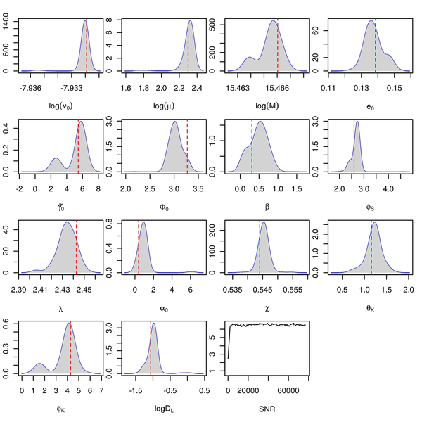
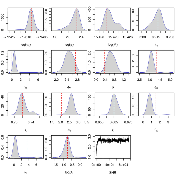
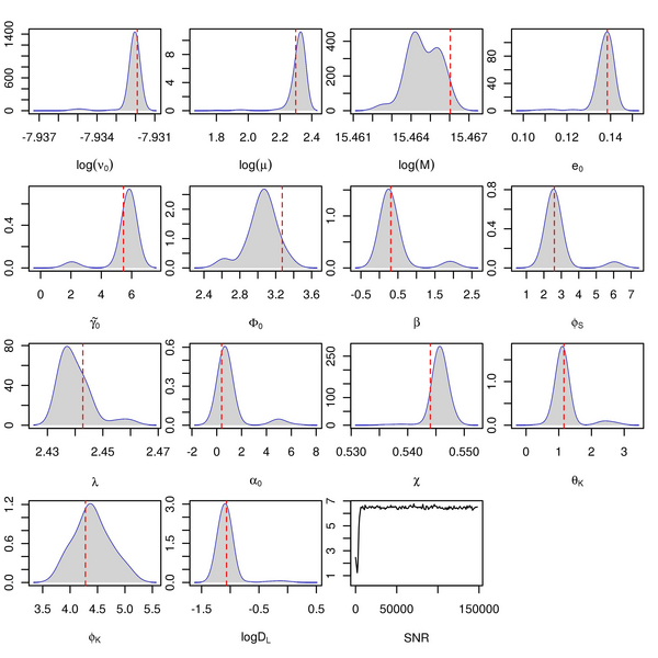
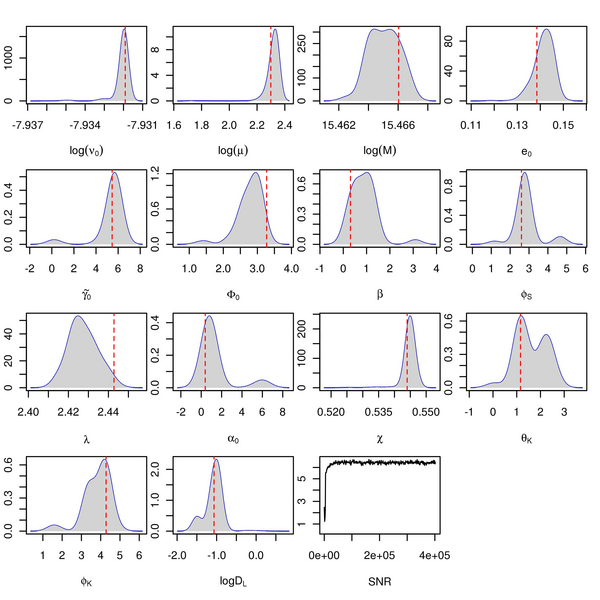
Density Plots

This was a short run i.e. less than 150K iterations with 30 chains PTMCMC. Here are the density plots for the coldest chain.

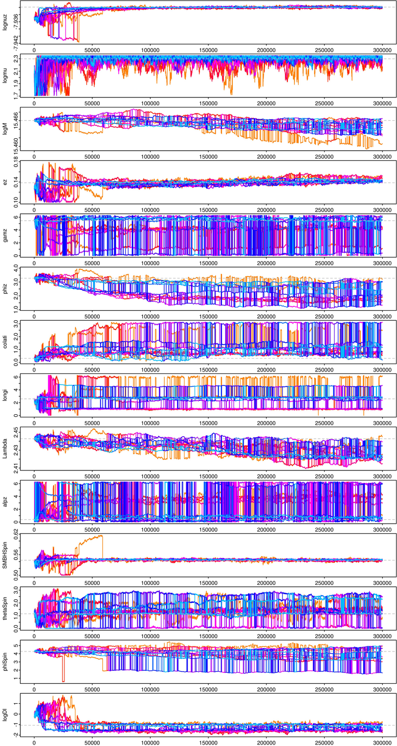
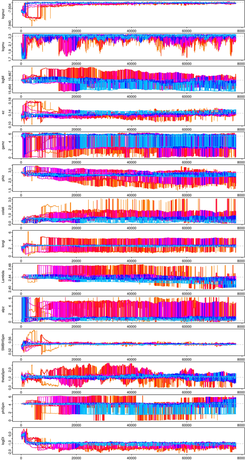
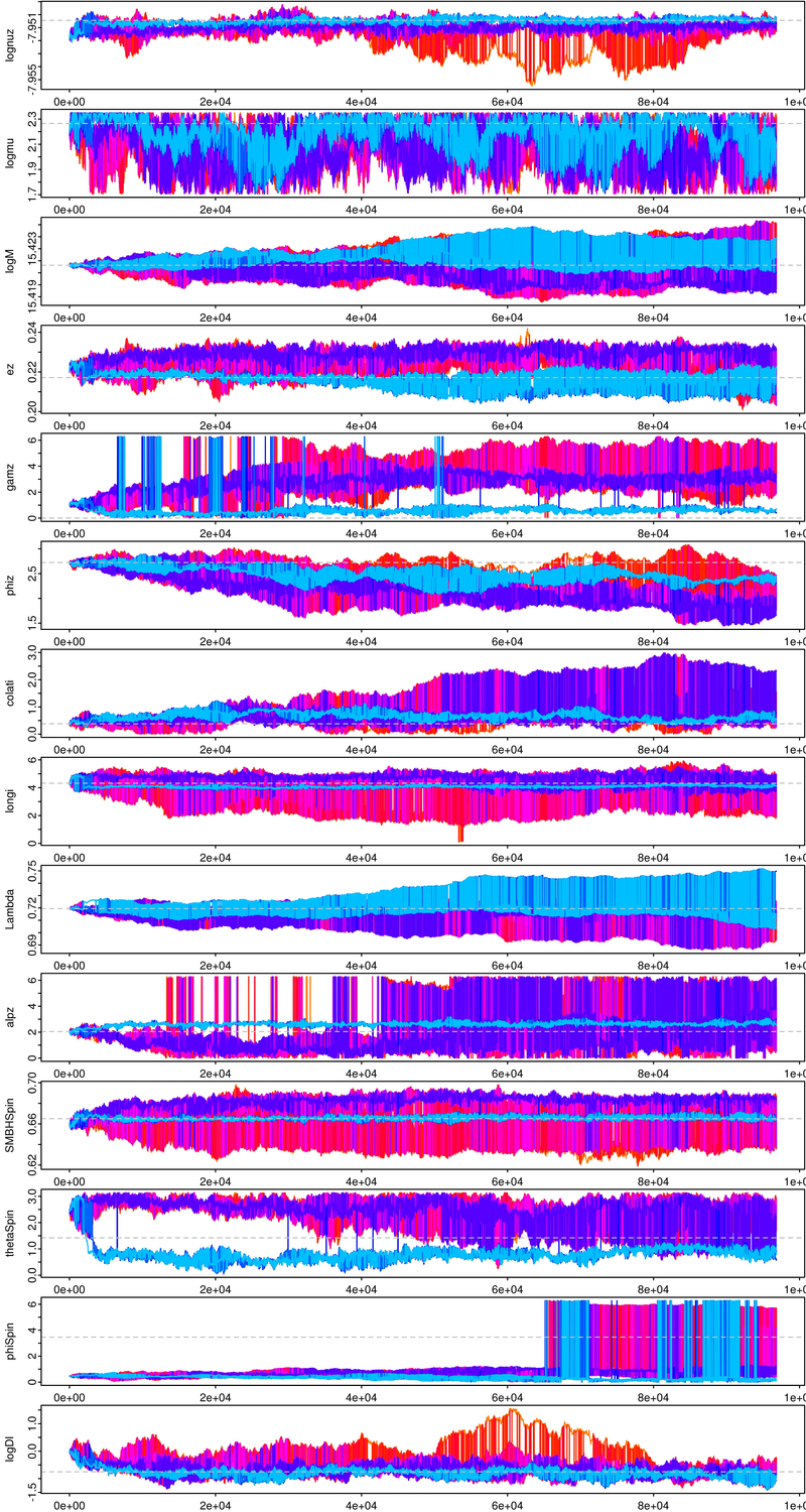
Trace plots of the first 10 chains only

The trace plots for the first 10 chains are given in the following figure the rest of 20 were not plotted because then the plot becomes too messy and nothing can be seen clearly.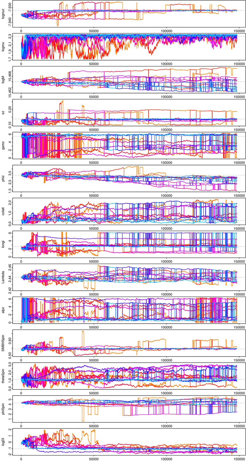

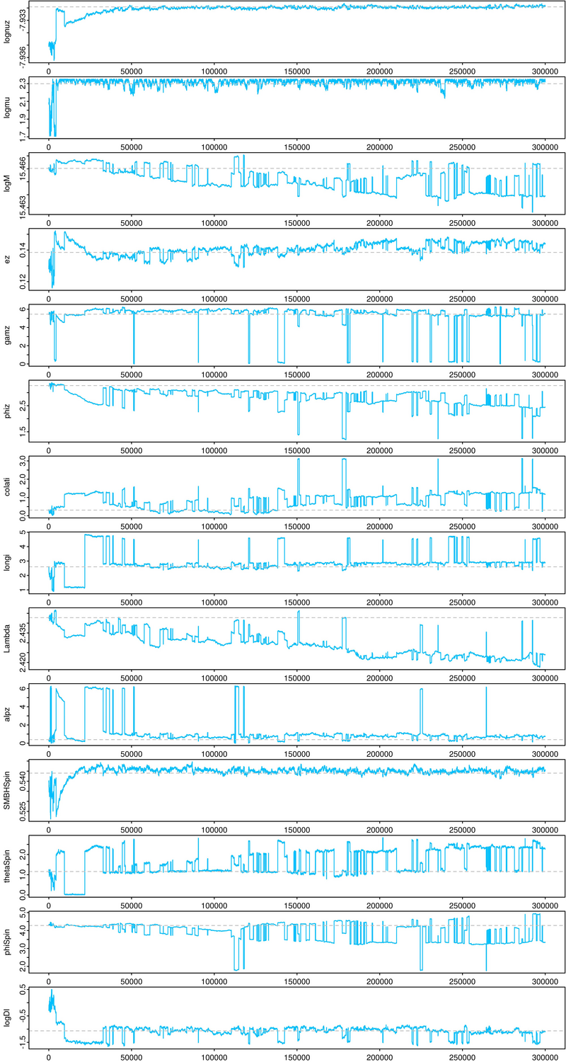
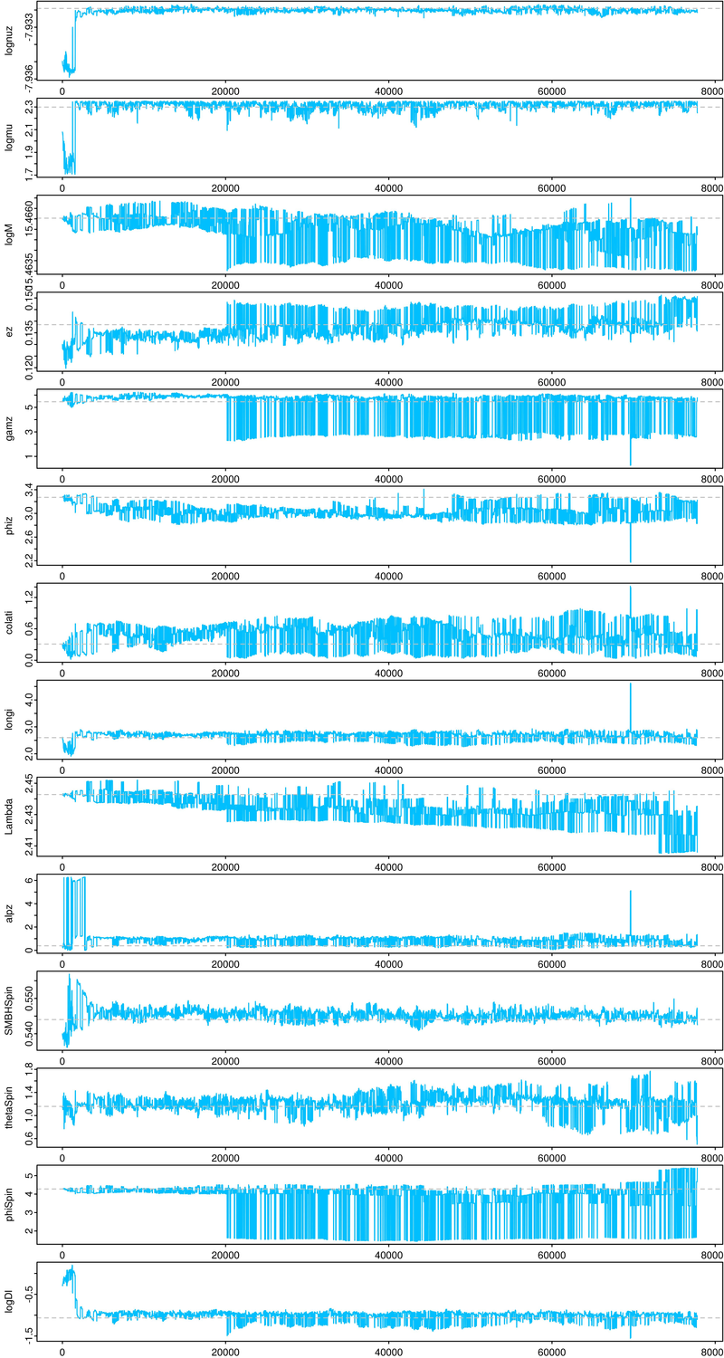
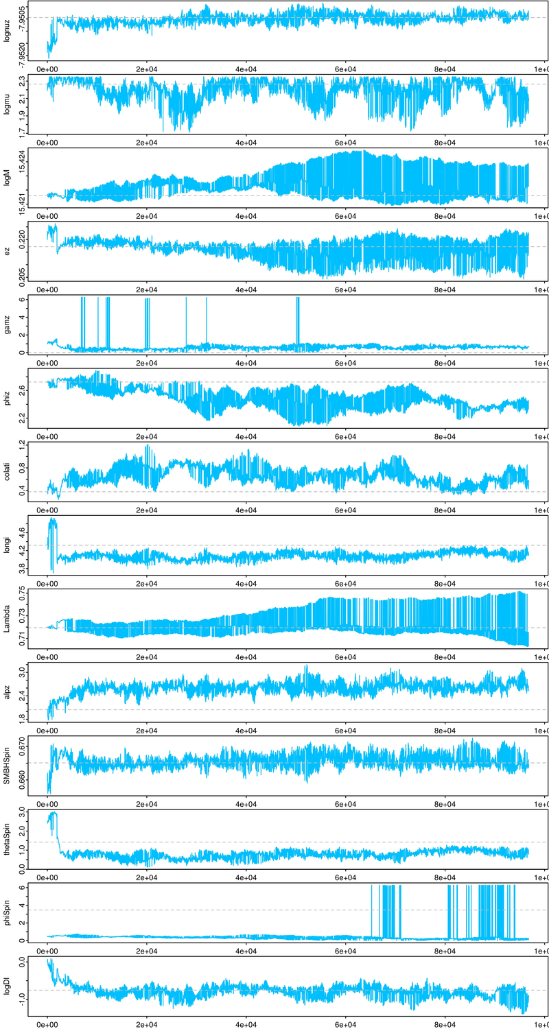
Trace plots of the first (coldest) chain

This above multiple chains plot still looks like a mess but for most of the key parameters most of chains are converged. If we plot the first five chains then they will be looking like a single chain. The hotter chains does not stay at one mode they keep moving here and there helping colder chains to settle. Following is the traceplot for the coldest chain.

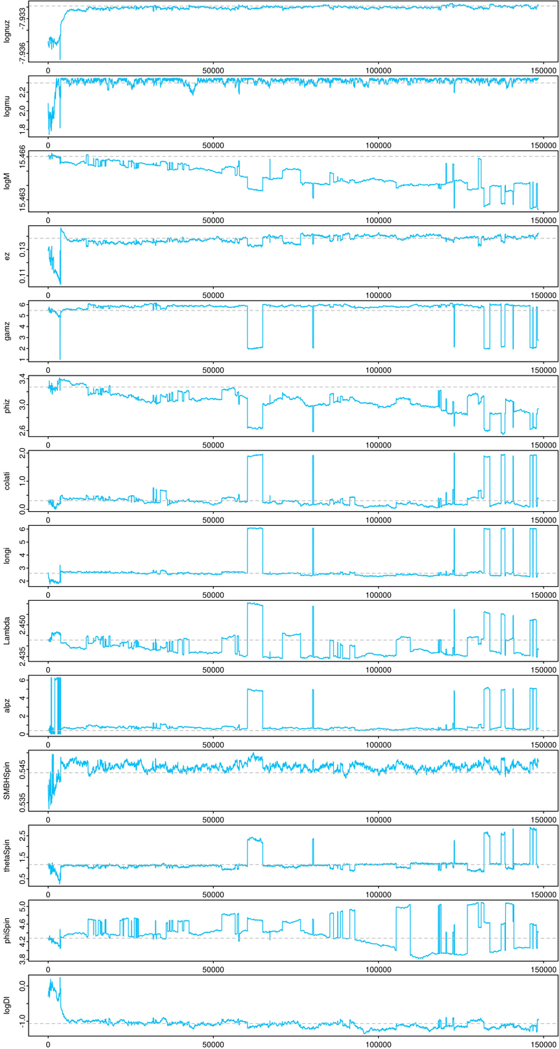
Trace plots of the first (coldest) chain

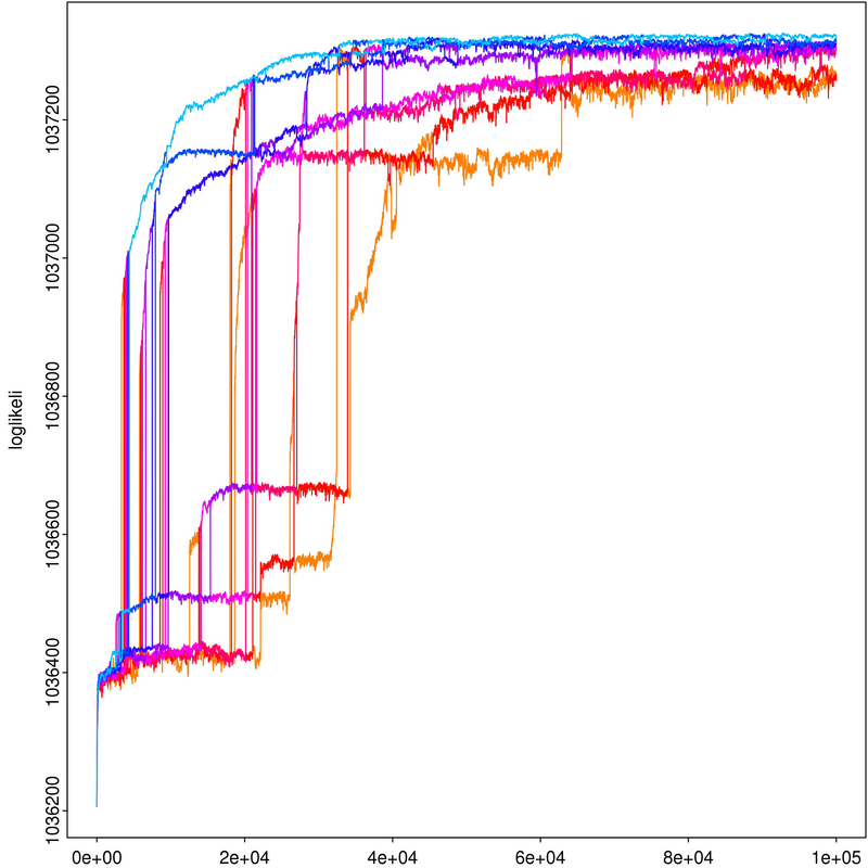
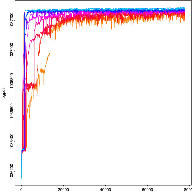
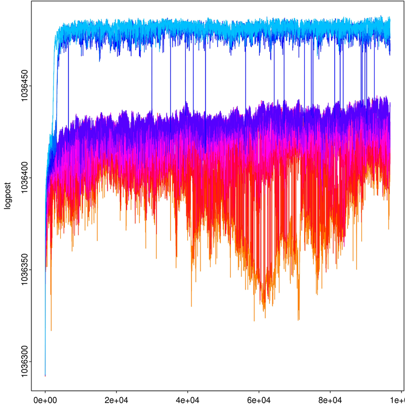
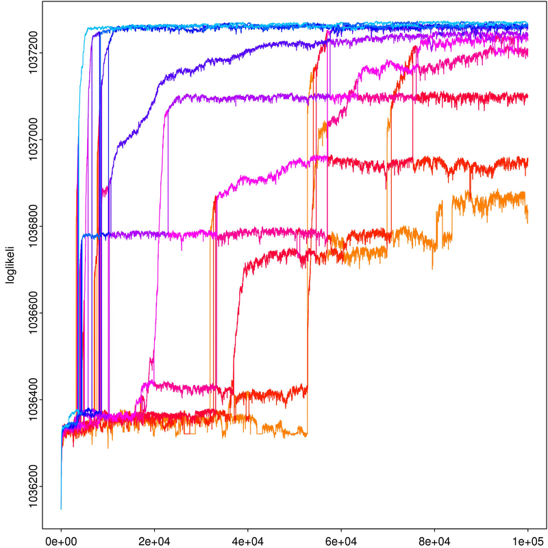
The log-likelihood behaviour at different temperatures is depicted in the following figure. This is actually a zoomed part of the log-likelihood traceplot and it shows how are different chains exchanging information at some points and how is the code progressing towards a global mode.

First signal : A longer MCMC run

Following denisty and trace plots are of the same signal as above but is a little longer MCMC run. In longer run the code behaviour gets improved.

Density Plots

Trace plots of the first 10 chains only

Trace plots of the first (coldest) chain

Likelihood history plots

The same first signal: Applying temperature to the whole posterior instead of likelihood only

Following are the results when tempearture was applied to the whole posterior instead of likelihood only. This was again 30 chians MCMC run. If we compare these density and trace plots to the above plots we can see a clear difference. The estimation accuarcy is increased as can be seen from the density plots.

Density Plots

Trace plots of the first 10 chains

Trace plots of the first (coldest) chain

Posterior history plots

If we compare this plot to its counterparts (likelihood history) as given above we can see a clear difference between them. Here all the posteriors quickly gets to the the same mode, despite the same starting values, temperature steps, and proposal distributions as for the above MCMC runs.

Second Signal

A 10 chain MCMC was ran to see if it can dectect this second signal. This is a rather weaker signal in the sence of its true SNR which is much lower than the previous one. Its density and trace plots are as under and are self explanatory. Also here I applied temperature to full posterior instead of only tempering the likelihood part.

The following plot shows the logposterior plot, which shows an upward moment as the parameters gets getter and better. Since here we applied lesser temperature the behaviour is not as good as the previous signal.