<?xml version="1.0" encoding="UTF-8"?>
<html>
  <head>
    <style type="text/css">
    @media print {
      body { }
      p.img { text-align: center; page-break-inside: avoid }
      img.CC { display: inline }
    }
    @media screen {
      body { max-width: 800px; margin: auto }
      p.img { text-align: center }
      img.CC { display: inline }
    }
    p.date {
      font-size: smaller;
      margin: 0;
    }
    p.versionHistory {
      color: gray
    }
    p.versionHistory a {
      color: gray
    }
    p.ref {
      text-indent: -2em;
      padding-left: 2em;
    }
  </style>
    <!-- PDFjs code (more at the end of the document) -->
    <script src="https://mozilla.github.io/pdf.js/build/pdf.js"/>
  </head>
  <body>
    <h1>Rendering HTML Content in R Graphics</h1>
    <p>
      <span style="font-style: italic">by Paul Murrell</span>
      <a href="http://orcid.org">
        <img alt="" src="https://www.stat.auckland.ac.nz/~paul/ORCID/ORCiD.png" style="width: 16px; height: 16px; vertical-align: middle"/>
      </a>
      <span style="font-family: mono; font-size: small">
        <a href="http://orcid.org/0000-0002-3224-8858">http://orcid.org/0000-0002-3224-8858</a>
      </span>
    </p>
    <p class="date">
    Version 3:
    <rcode echo="FALSE" results="asis"><![CDATA[
cat(format(Sys.Date(), "%A %d %B %Y"))
    ]]></rcode>
  </p>
    <p class="date versionHistory">
    Version 1:  original publication<br/>
    Version 2:  fixed up 'gridExtra' citation<br/>
    Version 3:  update pdf.js code (for displaying PDFs)
  </p>
    <rcode id="init" echo="FALSE" message="FALSE" results="hide"><![CDATA[
opts_chunk$set(comment=" ", tidy=FALSE)
options(width=100)
## For wonky desktop set up
options(bitmapType="cairo")
  ]]></rcode>
    <rcode echo="FALSE"><![CDATA[
    library(grid)
  ]]></rcode>
    <hr/>
    <p><a rel="license" href="http://creativecommons.org/licenses/by/4.0/"><img class="CC" alt="Creative Commons License" style="border-width:0" src="https://i.creativecommons.org/l/by/4.0/88x31.png"/></a><br/><span xmlns:dct="http://purl.org/dc/terms/" property="dct:title">This document</span>
    by <span xmlns:cc="http://creativecommons.org/ns#" property="cc:attributionName">Paul
    Murrell</span> is licensed under a <a rel="license" href="http://creativecommons.org/licenses/by/4.0/">Creative
    Commons Attribution 4.0 International License</a>.
  </p>
    <hr/>
    <p>
    This report describes several R packages that allow
    HTML content to be rendered as part of an R plot.
    The core package is called 'layoutEngine', but that package requires
    a "backend" package to perform HTML layout calculations.
    Three example backends are demonstrated: 'layoutEngineCSSBox',
    'layoutEnginePhantomJS', and 'layoutEngineDOM'.
    We also introduce two new font packages, 'gyre' and 'courier'.
  </p>
    <div>
      <h2>Table of Contents:</h2>
      <ul style="list-style: none">
        <li>
          <a href="#intro">1. Introduction</a>
        </li>
        <li>
          <a href="#why">2. Why render HTML in R graphics?</a>
        </li>
        <li>
          <a href="#mixing">3. Mixing HTML and R Graphics</a>
        </li>
        <li>
          <a href="#fonts">4. Defining fonts</a>
        </li>
        <li>
          <a href="#low-level">5. The lower-level interface</a>
        </li>
        <li>
          <a href="#backends">6. 'layoutEngine' backends</a>
        </li>
        <li>
          <a href="#limitations">7. Limitations</a>
        </li>
        <li>
          <a href="#discussion">8. Discussion</a>
        </li>
        <li>
          <a href="#requirements">9. Technical requirements</a>
        </li>
        <li>
          <a href="#Resources">10. Resources</a>
        </li>
        <li>
          <a href="#references">11. References</a>
        </li>
      </ul>
    </div>
    <h2>
      <a name="intro">1. Introduction</a>
    </h2>
    <p>
    The aim of the 'layoutEngine' package is to support rendering of HTML 
    content
    within R graphics (<a href="#R">R Core Team, 2018</a>).
    The following code provides a simple demonstration.
    We start with a standard 'lattice' plot (<a href="#pkg:lattice">Sarkar, 2008</a>).
  </p>
    <rcode><![CDATA[
library(lattice)
  ]]></rcode>
    <rcode id="xyplot" eval="FALSE"><![CDATA[
xyplot(mpg ~ disp, mtcars)
  ]]></rcode>
    <p>
    Next, we generate some HTML, in this case using <code>xtable</code> 
    from the 'xtable' package (<a href="#pkg:xtable">Dahl, 2016</a>).
  </p>
    <rcode><![CDATA[
library(xtable)
html <- print(xtable(head(mtcars[1:3])), type="html", print.results=FALSE)    
  ]]></rcode>
    <p>
    Finally, we navigate to the main 'lattice' panel viewport
    and call <code>grid.html</code> from the 'layoutEngine' package 
    (<a href="#pkg:layoutengine">Murrell, 2018d</a>),
    using the 'layoutEnginePhantomJS' backend 
    (<a href="#pkg:layoutenginephantomjs">Murrell, 2018g</a>),
    to render the HTML table (in the top right corner of the plot).
  </p>
    <rcode message="FALSE"><![CDATA[
library(layoutEnginePhantomJS)
  ]]></rcode>
    <rcode id="latticetable" eval="FALSE" results="hide"><![CDATA[
downViewport("plot_01.panel.1.1.vp")
grid.html(html, 
          x=unit(1, "npc") - unit(2, "mm"),
          y=unit(1, "npc") - unit(2, "mm"),
          just=c("right", "top"))    
  ]]></rcode>
    <rcode echo="FALSE" dpi="96" results="hide" warning="FALSE"><![CDATA[
<<xyplot>>
<<latticetable>>
  ]]></rcode>
    <p>
    We could do the same thing in a single step using a 'lattice'
    "panel function".  The following code produces exactly the same result
    as the plot above.
  </p>
    <rcode fig.keep="none" warning="FALSE"><![CDATA[
xyplot(mpg ~ disp, mtcars,
       panel=function(...) {
           panel.xyplot(...)
           grid.html(html, 
                     x=unit(1, "npc") - unit(2, "mm"),
                     y=unit(1, "npc") - unit(2, "mm"),
                     just=c("right", "top"))    
       })
  ]]></rcode>
    <p>
    The next two sections describe the main functions in the 
    'layoutEngine' package through a series of examples.
    Subsequent sections go into the underlying design details
    of the package.
  </p>
    <!--
  <p>
    PNG version ...
    NOTE that it is best to set the PNG resolution to 96 (because ... ?)
  </p>
  <rcode echo="FALSE" warning="FALSE" results="hide" fig.keep="none"><![CDATA[
res <- 96
png("lattice.png", res=res, width=res*7, height=res*7)
<<xyplot>>
<<latticetable>>
dev.off()
  ]]></rcode>
  <p>
    <img src="lattice.png"/>
  </p>
  <rcode echo="FALSE" results="hide" fig.keep="none"><![CDATA[
cairo_pdf("lattice-cairo.pdf")
<<xyplot>>
<<latticetable>>
dev.off()
  ]]></rcode>
  <p>
    Cairo PDF version ...
  </p>
  <canvas id="lattice-cairo" class="pdf"></canvas>
  <rcode echo="FALSE" results="hide" fig.keep="none"><![CDATA[
pdf("lattice.pdf")
<<xyplot>>
<<latticetable>>
dev.off()
embed_fonts("lattice.pdf")
  ]]></rcode>
  <p>
    PDF version ...
  </p>
  <canvas id="lattice" class="pdf"></canvas>
-->
    <h2>
      <a name="why">2. Why render HTML in R graphics?</a>
    </h2>
    <p>
    One reason for creating the 'layoutEngine' package is to
    be able to generate graphics that are easy (or easier) to describe
    in HTML compared to R graphics.
  </p>
    <p>
    For example, in R graphics, we can normally only draw text with a single
    font face.  The following code uses <code>grid.html</code>
    to draw text containing plain, <em>italic</em>, and <strong>bold</strong>
    font faces.
  </p>
    <rcode results="hide" dpi="96" fig.width="3" fig.height=".5"><![CDATA[
grid.html("<p>plain, <em>italic</em>, and <strong>bold</strong></p>")
  ]]></rcode>
    <p>
    The above example is actually possible in R graphics if we
    (mis)use a mathematical expression, like this ...
  </p>
    <pre>
grid.text(expression(paste("plain, ", italic(italic), ", and ", bold(bold))))
  </pre>
    <p>
    ... but something that really is not possible in R graphics is the
    use of more than one font <em>family</em> in a single piece of text.  The
    following code shows how we can do this with
    <code>grid.html</code>.
  </p>
    <rcode results="hide" dpi="96" fig.width="3" fig.height=".5"><![CDATA[
Rfonts <- c("sans", "serif", "mono", "Carlito")
CSSfonts <- cssFontFamily(Rfonts)
grid.html(paste0('<p><span style="font-family: ', CSSfonts["sans"], 
                     '">sans</span>, ',
                 '   <span style="font-family: ', CSSfonts["serif"], 
                     '">serif</span>, ',
                 '   <span style="font-family: ', CSSfonts["mono"], 
                     '">mono</span>, and ',
                 '   <span style="font-family: ', CSSfonts["Carlito"],
                     '">Carlito</span>.'),
          fonts=Rfonts)
  ]]></rcode>
    <p>
    The code above demonstrates an important point about using
    <code>grid.html</code>.  If we are rendering HTML that includes text
    content, we must specify the fonts that we are using for that text.
    This font specification must happen in R, via the <code>fonts</code>
    argument to <code>grid.html</code>, 
    and in CSS within the HTML that we are rendering, 
    typically via <code>style</code> attributes,
    <em>and</em> those specifications must match.  The 
    <code>cssFontFamily</code> function can be used to map R fonts
    to CSS fonts to make sure that we are specifying the same font in
    both R and CSS.  The Section on <a href="#fonts">Defining fonts</a> contains much more
    information on this topic.  We did not have to specify any fonts in the 
    previous examples because <code>grid.html</code> defaults to using
    a <code>"sans"</code> font.
  </p>
    <p>
    The introduction showed another example use of 'layoutEngine',
    which is to take advantage of the typesetting features of HTML
    to arrange text in a table, especially when packages like 'xtable'
    have already
    been written to generate the required HTML.
    The following code shows a more complex table example 
    from the 'formattable' package (<a href="#pkg:formattable">Ren and Russell, 2016</a>).
  </p>
    <!--
    https://cran.r-project.org/web/packages/formattable/vignettes/formattable-data-frame.html
  -->
    <rcode message="FALSE"><![CDATA[
library(formattable)
  ]]></rcode>
    <rcode><![CDATA[
products <- data.frame(id = 1:5, 
  price = c(10, 15, 12, 8, 9),
  rating = c(5, 4, 4, 3, 4),
  market_share = percent(c(0.1, 0.12, 0.05, 0.03, 0.14)),
  revenue = accounting(c(55000, 36400, 12000, -25000, 98100)),
  profit = accounting(c(25300, 11500, -8200, -46000, 65000)))    
  ]]></rcode>
    <rcode><![CDATA[
sign_formatter <- formatter("span", 
  style = x ~ style(color = ifelse(x > 0, "green", 
    ifelse(x < 0, "red", "black"))))
  ]]></rcode>
    <rcode><![CDATA[
table <- formattable(products, list(
  price = color_tile("transparent", "lightpink"),
  rating = color_bar("lightgreen"),
  market_share = color_bar("lightblue"),
  revenue = sign_formatter,
  profit = sign_formatter))
  ]]></rcode>
    <rcode dpi="96" fig.width="5" fig.height="3"><![CDATA[
grid.html(as.character(table))
  ]]></rcode>
    <p>
    The result of the rendering in the example above is not exactly the same
    as the rendering that a browser produces.  The layout of the table 
    is correct and the colours are correct, but in the browser the
    coloured backgrounds are rounded rectangles (because the
    HTML that 'formattable' generated uses the CSS
    property <code>border-radius</code>).  This imperfect rendering reflects 
    the fact that the 'layoutEngine' package currently only supports
    some basic CSS properties.  For much more information on the limitations
    of the 'layoutEngine' package, see the <a href="#discussion">Discussion</a> Section.
  </p>
    <p>
    In a <a href="https://www.displayr.com/pure-html/?utm_medium=Feed&amp;utm_source=Syndication">DisplayR Blog post</a>, Tim Bock extolls 
    the relative simplicity of 
    generating tables in HTML, using an example that required wrapped text
    for both row and column headers.  In his post, he provided code for
    generating the HTML table from R;  the following code renders that
    HTML code back in R graphics.
  </p>
    <rcode dpi="96" fig.height="5"><![CDATA[
options(layoutEngine.backend=phantomjsEngine)
html <- readLines("displayr.html")
htmlDoc <- htmlDocument(html)
grid.html(htmlDoc)
  ]]></rcode>
    <p>
    The new feature in the code above is a call to the <code>htmlDocument</code>
    function.  This alternative to the <code>htmlElement</code> function
    is intended
    for when we have a complete HTML document (rather than just 
    an HTML fragment) that we want to render in R.  We have to call
    <code>htmlDocument</code> explicitly because <code>grid.html</code>
    assumes that character input is only an HTML fragment (and 
    calls <code>htmlElement</code> itself).
  </p>
    <p>
    Drawing tables of values can be achieved
    directly in R graphics 
    (e.g., using <code>grid.table</code> from the 'gridExtra' package; 
    <a href="#pkg:gridExtra">Auguie, 2017</a>),
    but HTML (combined with CSS) provides many other typesetting 
    features that are not covered by R graphics packages.
    The following code shows an example of the CSS <code>shape-outside</code>
    property
    (combined with the <code>float</code> property), which allows us to 
    flow text around a non-rectangular shape (in this case a circle).
  </p>
    <p>
    For this example, we switch to the 'layoutEngineDOM' backend 
    (<a href="#pkg:layoutenginedom">Murrell, 2018f</a>)
    because the 'layoutEnginePhantomJS' backend does not support
    the <code>shape-outside</code> property.  The 'layoutEngineDOM'
    backend provides access to the default system web browser (which
    is a recent Firefox for this report), which means that we can gain access
    to the most recent CSS properties.
  </p>
    <rcode id="circle-flow" eval="FALSE"><![CDATA[
library(layoutEngineDOM)
## Give browser plenty of time to do its work
options(DOM.limit=10)
html <- c('<div style="width: 350px; border-width: 1px; border-style: solid">',
          '<div style="background-color: #7db9e8;
                       width: 200px; height: 200px;
                       float: right; shape-outside: circle()"/>',
          '<p>This text flows around a circle! Try doing that
              in R!</p>',
          '</div>')
  ]]></rcode>
    <rcode eval="FALSE"><![CDATA[
grid.html(html)
  ]]></rcode>
    <rcode dpi="96" echo="FALSE" fig.width="4" fig.height="3"><![CDATA[
<<circle-flow>>
grid.html(html, viewports=TRUE)
grid.force()
downViewport("BODY.1.DIV.2.DIV.2.vp")
grid.circle(gp=gpar(fill=NA))
  ]]></rcode>
    <h2>
      <a name="mixing">3. Mixing HTML and R Graphics</a>
    </h2>
    <p>
    The real value of being able to render HTML content in R is not
    just so that we can reproduce what would appear in a browser.
    This facility becomes more useful when we combine the HTML content
    with other graphical output that R is good at, such as plots.
    An example of this was shown in the introduction, where an HTML
    table was drawn within a 'lattice' plot.  This section demonstrates
    some other possibilities.
  </p>
    <p>
    The code below uses HTML rendering to provide a plot axis label
    for a 'lattice' plot that contains more than one font 
    (the R variable name is drawn with a typewriter font).
    One difference about this code is the use of 
    <code>htmlGrob</code> rather than <code>grid.html</code>
    because we need to specify the label to <code>xyplot</code> as a 
    'grid' grob (rather than just draw it immediately).
    We also call the <code>flow</code> function to lay out the HTML content
    and pass that to <code>htmlGrob</code> (rather than passing the
    raw HTML).  This is because <code>xyplot</code> queries the
    label grob several times (e.g., for its height and width) and we do
    not want to have to perform the HTML layout for every query.
    The Section on <a href="#low-level">The lower-level interface</a> discusses the <code>flow</code>
    function in more detail.
  </p>
    <!-- phantomjsEngine gets this wrong (width of 'disp' is WAY too large)
       for some reason - not sure why yet 
  -->
    <p>
    For this example, we switch to the CSS Box backend, 'layoutEngineCSSBox' 
    (<a href="#pkg:layoutenginecssbox">Murrell, 2018e</a>).  We use this backend for
    this example because it produces a better result than
    the PhantomJS backend and it is "quieter" than the 'DOM' backend.
    The Section on <a href="#backends">'layoutEngine' backends</a> discusses the strengths
    and weaknesses of the different backends in more detail.
  </p>
    <rcode dpi="96"><![CDATA[
library(layoutEngineCSSBox)
html <- paste0('<span>Engine Displacement ',
               '  (<span style="font-family: ', CSSfonts["mono"], '">disp</span>)',
               "</span>")
flowedHTML <- flow(html)
xyplot(mpg ~ disp, mtcars, xlab=htmlGrob(flowedHTML))
  ]]></rcode>
    <p>
    The next example, from a <a href="https://stackoverflow.com/questions/47186918/ggplot-italicize-part-of-caption-and-divide-text-over-two-lines/47189718#47189718">Stack Overflow</a> post,
    is very similar.  This example involves adding a caption to a 
    'ggplot2' plot (<a href="#pkg:ggplot2">Wickham, 2016</a>), using
    <code>gridExtra::grid.arrange</code> to arrange the
    plot above the caption.
    The caption 
    does not involve multiple font families, but 
    it does involve multiple font faces <em>and</em> it involves
    text split across two lines
    (which is a step too far for R's limited plotmath facility).
    This is a good example of a typesetting task that looks very simple,
    and is simple in HTML, but is not normally possible in R graphics.
  </p>
    <rcode><![CDATA[
library(ggplot2)
library(gridExtra)
  ]]></rcode>
    <rcode dpi="96"><![CDATA[
note <- '
    <p style="font-size: 7.5pt; line-height: 0.8">
      <span style="font-style: italic">Note: </span> 
      Market concentration averages in the United States, 
      United Kingdom, and the <br>
      Netherlands are, respectively, 1920, 1388, and 1244
    </p>
'
gg <- ggplot(mtcars, aes(wt, mpg)) + geom_point()
caption <- htmlGrob(flow(note))
grid.arrange(gg, bottom=caption)
  ]]></rcode>
    <p>
    The next example demonstrates that, having rendered HTML content
    in R (with 'grid') in combination with an R plot (based on 'grid'),
    it is possible to make use of 'grid' tools to further integrate the
    HTML output with the R plot output.
    In the following code, we draw a 'lattice' plot, add an HTML
    table at the top-right of the plot, then draw an arrow from the
    left edge of a piece of text within the HTML table to the corresponding
    data point within the 'lattice' plot.
  </p>
    <rcode dpi="96" warning="FALSE"><![CDATA[
options(layoutEngine.backend=phantomjsEngine)
xyplot(mpg ~ disp, mtcars)
html <- print(xtable(head(mtcars[1:3])), type="html", print.results=FALSE)    
flowedhtml <- flow(html)
downViewport("plot_01.panel.1.1.vp")
grid.html(flowedhtml, 
          x=unit(1, "npc") - unit(2, "mm"),
          y=unit(1, "npc") - unit(2, "mm"),
          just=c("right", "top"),
          viewports=TRUE)    
grid.move.to(mtcars$disp[1], mtcars$mpg[1], default.units="native")
upViewport(0)
vp <- grid.grep("TD.+SPAN.+vp", grep=TRUE, viewports=TRUE)
downViewport(vp)
arr <- arrow(ends="first", angle=15, length=unit(5, "mm"), type="closed")
grid.line.to(unit(-1, "mm"), .5, arrow=arr, gp=gpar(fill="black"))
  ]]></rcode>
    <p>
    There are a couple of interesting features in the code above.
    One new feature is the use of <code>viewports=TRUE</code> in the
    call to <code>grid.html</code>.  This means that, in addition to
    drawing the HTML content, 'grid' viewports are created that correspond
    to each piece of HTML content.  This is what allows us to use
    <code>grid.grep</code> to find the viewport that corresponds to
    the first &lt;SPAN&gt; element within a &lt;TD&gt; element 
    within the HTML table (so that we can navigate down to that viewport
    to specify one end of the arrow).
  </p>
    <p>
    Another feature is the use of the <code>flow</code> function.
    The reason for calling <code>flow</code> in this example
    is slightly different than the previous one.  This time we are making
    sure that the 'grid' grobs and viewports that are created when the
    HTML content is rendered are visible on the 'grid' display list
    (so that we can navigate to the viewports that correspond to the 
    HTML content to add drawing).  If we just passed the raw HTML directly
    to <code>grid.html</code>, we would have had to call <code>grid.force</code>
    (and trigger another HTML layout calculation) in order to make the
    'grid' grobs and viewports visible on the 'grid' display list.
    The Section on <a href="#low-level">The lower-level interface</a> explains the difference between
    flowed HTML and raw HTML in more detail.
  </p>
    <p>
    The next example also demonstrates the use of <code>viewports=TRUE</code>
    to generate 'grid' viewports from HTML content.
    This example is a variation on the example from the previous section
    that used <code>shape-outside</code> to flow text around a 
    non-rectangular shape.
    This time, rather than specifying a circle to flow text around,
    we will specify an image, and the image will be an R plot
    (a pie chart).  We specify a transparent background for the image
    because <code>shape-outside</code> flows text around the non-transparent
    component of the image.
  </p>
    <rcode results="hide"><![CDATA[
pie.sales <- c(0.12, 0.3, 0.26, 0.16, 0.04, 0.12)
png("assets/pie.png", width=200, height=200,
    bg="transparent")
par(mar=rep(0, 4))
pie(pie.sales, radius=.95, labels=NA)
dev.off()
  ]]></rcode>
    <p>
      <img src="assets/pie.png"/>
    </p>
    <p>
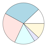
    The following code uses HTML to flow text around the pie chart, then
    navigates to the &lt;div&gt; that was flowed around and draws the
    R pie chart within the corresponding viewport.
  </p>
    <rcode dpi="96" fig.width="4" fig.height="3" results="hide"><![CDATA[
options(layoutEngine.backend=DOMEngine)
## Give browser plenty of time to do its work
options(DOM.limit=10)
html <- c('<div style="width: 350px; border-width: 1px; border-style: solid">',
          '<div id="pie"
                style="width: 200px; height: 200px;
                       float: right; shape-outside: url(assets/pie.png)"/>',
          '<p>Pie charts may not be the best data visualisation tool,
              but they are fantastic fun to flow text around!</p>',
          '</div>')
flowedhtml <- flow(html, assets=file.path(getwd(), "assets", "pie.png"))
grid.html(flowedhtml, viewports=TRUE)
vp <- grid.grep("pie", grep=TRUE, grobs=FALSE, viewports=TRUE)
downViewport(vp)
library(gridGraphics)
grid.echo(function() {
              par(mar=rep(0, 4))
              pie(pie.sales, radius=.95, labels=NA)
          },
          newpage=FALSE)
  ]]></rcode>
    <p>
    One interesting feature of the code above is that we have HTML content
    that refers to an external resource: the file <code>assets/pie.png</code>.
    In order to layout this sort of HTML, we must use the <code>assets</code>
    argument to <code>flow</code>, so that the layout engine can find
    the external resource.  This only applies when we are dealing with resources
    on the local file system;  external resources (URLs) should be resolved
    by the layout engine.  If we provide raw HTML directly to 
    <code>grid.html</code>, we can supply the <code>assets</code> argument there
    instead.
  </p>
    <p>
    Another detail about the code above is that we must use the 'gridGraphics'
    package (<a href="#pkg:gridGraphics">Murrell and Wen, 2018</a>) 
    to draw the pie chart because the 'layoutEngine' package
    works in the 'grid' graphics sytem and the <code>pie</code> function
    is based on the 'graphics' system.
  </p>
    <p>
    The next example further embraces the use of 'grid'
    viewports based on an HTML layout.  In this example, we use 
    CSS Grid Layout (<a href="#Atanassov:18:CGL">Atanassov et al., 2018</a>) 
    to produce an arrangement of regions 
    and then draw R plots within those regions.
    The following code describes HTML that contains
    a set of &lt;div&gt; elements,
    some of which are empty (we will use those to draw plots),
    and some of which contain text captions.  This is followed by
    CSS code that specifies the layout of the &lt;div&gt; elements,
    which consists of two columns and four rows, where the heights
    of the second and fourth rows are based on the size of the text captions.
  </p>
    <p>
    Having rendered this combination of HTML and CSS, we navigate to the
    empty &lt;div&gt; viewports and draw an R plot in each one.
    We switch back to the 'layoutEngineDOM' backend because we need
    support for CSS Grid Layouts.
  </p>
    <rcode dpi="96" dev.args="list(bg='transparent')" fig.width="5" fig.height="5"><![CDATA[
options(layoutEngine.backend=DOMEngine)
html <- '
  <div id="main">
    <div id="fig1"></div>
    <div id="fig2"></div>
    <div id="caption1">
      Figure 1: This caption takes up more than one row
    </div>
    <div id="caption2">
      Figure 2: This does not
    </div>
    <div id="fig3"></div>
    <div id="fig4"></div>
    <div id="caption3">
      Figure 3: One row
    </div>
    <div id="caption4">
      Figure 4: More than one row
    </div>
  </div>
'
css <- '
    div { 
      border-style: solid; 
      border-width: 1px; 
    }
    #main { 
      width: 400px;
      height: 400px;
      display: grid;
      grid-template-columns: 1fr 1fr;
      grid-template-rows: repeat(2, 1fr auto);
      grid-auto-flow: row;
    }
'
flowedhtml <- flow(html, css=css)
grid.html(flowedhtml, viewports=TRUE)
figvps <- grid.grep("fig", grep=TRUE, global=TRUE,
                    grobs=FALSE, viewports=TRUE)
for (i in 1:4) {
    downViewport(figvps[[i]])
    grid.echo(function() { par(mar=rep(0, 4)); pie(1:i, labels=NA) }, 
              newpage=FALSE)
    upViewport(0)
}
  ]]></rcode>
    <p>
    This layout would be tricky-to-impossible with a 'grid' layout because the
    heights of the second and fourth rows depend on the number of lines
    in the typeset text captions.
  </p>
    <p>
    A new feature in the code above is the 
    <code>css</code> argument in the call to <code>flow</code>.
    This is how we can provide CSS code separately from HTML code
    for laying out HTML content.
  </p>
    <p>
    The next example further emphasises the value of using a web browser
    as the backend.  In this example, we render a complete HTML page
    that contains a table that is styled and augmented by the 
    DataTables javascript library (<a href="#datatables">Jardine, 2014</a>).  
    Most of this result
    is just CSS, but the "3 of 3 entries" line below the table
    is generated by javascript code.  This demonstrates the idea
    that we can benefit from a backend that can evaluate javascript
    code to render HTML content that is (even partially) generated
    by a javascript library.
  </p>
    <rcode dpi="96" fig.height="3.5"><![CDATA[
htmlDoc <- htmlDocument(readLines("DataTable.html"))
grid.html(htmlDoc)
  ]]></rcode>
    <p>
    The final example really mixes things up.  This time, to generate
    HTML content, we use an (admittedly trivial)
    R Markdown document (shown below).
  </p>
    <rcode echo="FALSE"><![CDATA[
cat(readLines("example.Rmd"), sep="\n")
  ]]></rcode>
    <p>
    The 'rmarkdown' package (<a href="#pkg:rmarkdown">Allaire et al., 2017</a>) 
    is used to produce HTML,
    including running the embedded R code and including the R output
    in the final HTML,
    then that HTML is rendered at top-right within a 'lattice' plot.
  </p>
    <rcode eval="FALSE"><![CDATA[
library(rmarkdown)
render("example.Rmd", "html_document")
  ]]></rcode>
    <rcode echo="FALSE"><![CDATA[
## Run rmarkdown::render() in separate R process, rather than within
## a document that is already being knit()ed
system("Rscript -e 'library(rmarkdown); render(\"example.Rmd\", \"html_document\")'")    
  ]]></rcode>
    <!-- 'layoutEngineDOM' does not do well on this - perhaps because I am
       not setting up the fonts properly - in any case the fontBaseline() 
       calculation stuffs up and produces a large negative value (!) -->
    <rcode dpi="96" results="hide" message="FALSE"><![CDATA[
options(layoutEngine.backend=phantomjsEngine)
html <- readLines("example.html")
htmlDoc <- htmlDocument(html)
xyplot(mpg ~ disp, mtcars,
       panel=function(...) {
           panel.xyplot(...)
           grid.html(htmlDoc, 
                     x=unit(1, "npc") - unit(1, "mm"),
                     y=unit(1, "npc") - unit(1, "mm"),
                     width=unit(3, "in"),
                     just=c("right", "top"))
       })
  ]]></rcode>
    <p>
    This ends the high-level examples that demonstrate basic usage
    of the 'layoutEngine' package.  The remaining sections
    delve into the underlying design of the package and lower-level
    details of how things work.
  </p>
    <h2>
      <a name="fonts">4. Defining fonts</a>
    </h2>
    <p>
    A fundamental requirement of the 'layoutEngine' package is that
    exactly the same fonts are used both to layout HTML content in a backend
    engine (e.g., 'layoutEngineCSSBox') and to render the HTML content in R.
    This is a requirement because the layout of HTML content in almost all
    cases will depend on the typesetting of text within HTML containers
    (paragraphs, table cells, etc).  If the fonts do not match exactly,
    the rendered text in R will not align with other rendered HTML content
    (e.g., table borders). This section describes how this matching is
    achieved in the 'layoutEngine' package.
  </p>
    <p>
    Because the end goal is to render content in R graphics, we want to
    start with
    an R font specification and map that to a CSS font specification.
    A font specification in R consists of a font family name (e.g., "Carlito"),
    a font face (plain, bold, italic, or bold-italic), and a font size 
    (e.g., 12pt).
  </p>
    <p>
    In HTML, the font used for text can be controlled by the CSS 
    properties <code>font-family</code> (e.g., "Carlito"), 
    <code>font-weight</code> (e.g,
    "bold" or "normal"), <code>font-style</code> (e.g., "italic" or "normal"),
    and <code>font-size</code> (e.g., 12pt) (and 
    <code>font-variant</code>, but we are going to ignore that).
  </p>
    <p>
    The 'layoutEngine' package assumes that the HTML content that is 
    to be rendered either contains no font family information or only
    font families that map to R fonts
  </p>
    <p>
    A complication is the fact that 
    HTML and CSS are
    designed to be flexible with respect to fonts so that a web browser
    can render content with whatever fonts are available.  For example,
    the following CSS specification means that Helvetica will be used if
    it is available, then DejaVu Sans if it is available, then finally
    whatever sans-serif font the web browser can get its hands on.
  </p>
    <pre>
font-family: Helvetica, DejaVu Sans, sans
  </pre>
    <p>
    By contrast, 
    we want to tell the 'layoutEngine' backend to use an exact font,
    so instead we generate a CSS <code>@font-face</code> rule.  This allows
    us to specify an actual font file and associate it with a 
    font family and other properties.  For example, the following
    CSS specifies very precisely that the font family "TeXGyreHeros",
    with normal style and bold weight, corresponds to the font file
    found at the location <code>assets/qhvb.pfb</code> (relative to
    the location of the HTML document).
  </p>
    <pre>
@font-face {
  font-family: "TeXGyreHeros";
  font-style:  normal;
  font-weight: bold;
  src:         url('assets/qhvb.pfb');
}
  </pre>
    <p>
    In order to generate an <code>@font-face</code> rule, we need to
    know the location of the font file that we want to use.
    The 'layoutEngine' package makes use of the 'gdtools' package 
    (<a href="#pkg:gdtools">Gohel et al., 2018</a>)
    and the 'extrafont' package (<a href="#pkg:extrafont">Chang, 2018</a>) to achieve this.
  </p>
    <rcode results="hide" message="FALSE"><![CDATA[
library(gdtools)
library(extrafont)
  ]]></rcode>
    <p>
    The <code>sys_fonts</code> function from the 'gdtools' package
    is useful because it provides information about system fonts,
    including the location of font files.
  </p>
    <rcode echo="FALSE"><![CDATA[
options(width=100)
  ]]></rcode>
    <rcode><![CDATA[
sf <- sys_fonts()
head(sf[c("family", "weight", "slant", "file")])
  ]]></rcode>
    <rcode echo="FALSE"><![CDATA[
options(width=80)
  ]]></rcode>
    <p>
    This is useful for rendering HTML on R graphics devices that are
    based on <a href="https://www.cairographics.org/">Cairo graphics</a> 
    (<a href="#cairo">Packard et al., 2018</a>), such as the default screen device
    on Linux and the <code>cairo_pdf</code> device, because on those devices
    we can specify a system font just by its family name (e.g., "Gillius ADF";
    look at the 'g' in the output below).
  </p>
    <rcode results="hide"><![CDATA[
cairo_pdf("cairo-font.pdf", width=1, height=.5)
grid.text("Testing", gp=gpar(fontfamily="Gillius ADF"))
dev.off()
  ]]></rcode>
    <canvas id="cairo-font" class="pdf"/>
    <p>
    Unfortunately, specifying fonts on the standard <code>pdf</code> 
    graphics device (and the <code>postscript</code> device) is less
    straightforward;  we have to use the <code>Type1Font</code> function
    to associate
    AFM files with a font family name and then call <code>pdfFonts</code>
    (or <code>postscriptFonts</code>) to register the font for use with R.
    The 'extrafont' package makes this easier with its functions
    <code>font_import</code> and <code>loadfonts</code>, which automatically
    register system fonts.  The <code>fonttable</code> function can then
    be used to provide information about registered fonts, including
    the locations of font files.
  </p>
    <rcode echo="FALSE"><![CDATA[
options(width=100)
  ]]></rcode>
    <rcode><![CDATA[
ft <- fonttable()
head(ft[c("FamilyName", "Bold", "Italic", "fontfile")])
  ]]></rcode>
    <rcode echo="FALSE"><![CDATA[
options(width=80)
  ]]></rcode>
    <p>
    The only problem is that 'extrafont' only registers TrueType system fonts.
    However, 'extrafont' also provides a <code>font_install</code> function that
    can be used to load special font packages and those can contain
    Type 1 fonts.  As examples, the 
    'gyre' package (<a href="#pkg:gyre">Murrell, 2018c</a>) has been created to bundle the
    TeX Gyre fonts 
    (<a href="#Hagen:TB27-2-230">Hagen et al., 2006</a>, <a href="#Hefferon:TB30-2-236">Hefferon, 2009</a>) 
    and the 'courier' package (<a href="#pkg:courier">Murrell, 2018a</a>) bundles
    the IBM Courier font (<a href="#IBMcourier">IBM Corporation, 1990</a>).
  </p>
    <p>
    The following code repeats the text-with-multiple-font-families
    example from earlier, but performs the rendering on the standard
    <code>pdf</code> device.  This requires the 'gyre' and 'courier'
    packages to be loaded.  Notice also that the mappings from R fonts
    to CSS fonts has to be recalculated because we are rendering
    to a different graphics device than before.
  </p>
    <rcode results="hide"><![CDATA[
library(gyre)
library(courier)    
  ]]></rcode>
    <rcode fig.keep="none" results="hide"><![CDATA[
pdf("multifont.pdf", width=3, height=.5)
CSSfontsPDF <- cssFontFamily(Rfonts)
grid.html(paste0('<p><span style="font-family: ', CSSfontsPDF["sans"], 
                     '">sans</span>, ',
                 '   <span style="font-family: ', CSSfontsPDF["serif"], 
                     '">serif</span>, ',
                 '   <span style="font-family: ', CSSfontsPDF["mono"], 
                     '">mono</span>, and ',
                 '   <span style="font-family: ', CSSfontsPDF["Carlito"],
                     '">Carlito</span>.'),
          fonts=Rfonts)
dev.off()
embed_fonts("multifont.pdf")
  ]]></rcode>
    <canvas id="multifont" class="pdf">
  </canvas>
    <p>
    A final wrinkle is that in R it is possible to specify one of three
    generic font families: "sans", "serif", and "mono".
    In order to map these to a specific font (that both R and CSS will use),
    the 'layoutEngine' package uses <code>match_family</code> from the
    'gdtools' package (on Cairo-based devices,
    this is after first mapping "sans" to "Helvetica", "serif" to
    "Times", and "mono" to "Courier", to match what R graphics 
    does internally).  
  </p>
    <p>
    The <code>cssFontFamily</code> function from the
    'layoutEngine' package can be used to show how an R font family
    maps to a CSS <code>font-family</code>, though the mapping is
    dependent on the graphics device in use.
  </p>
    <rcode><![CDATA[
cssFontFamily(c("sans", "serif", "mono"), device="pdf")
cssFontFamily(c("sans", "serif", "mono"), device="cairo_pdf")
  ]]></rcode>
    <p>
    In summary, when we call <code>grid.html</code> (or <code>flow</code>),
    we must specify which fonts we want to use by providing one or more
    R font family names (the default is just "sans").  These
    font family names are converted to CSS <code>@font-face</code> rules
    that associate a CSS <code>font-family</code> with an exact font file.
    For this to work (because we need paths to font files), 
    we must only use R font family names that exist 
    within the <code>gdtools::sys_fonts</code> font table (for Cairo-based
    devices) or within the <code>extrafont::fonttable</code> font table
    (for <code>pdf</code> or <code>postscript</code>).  For cairo-based
    devices we should be able to use any system font.  For <code>pdf</code>
    or <code>postscript</code> we can use any TrueType system font
    and we can add further Type 1 fonts creating
    a font package or making use of an existing font package
    like 'gyre' or 'courier'.
  </p>
    <p>
    When we are working with a <code>pdf</code> or <code>postscript</code>
    graphics device, it is a good idea to embed fonts in the final document
    (using <code>extrafont::embed_fonts</code>), otherwise we risk all 
    of our hard work being undone if a PDF viewer cannot find the fonts
    that we have used and is forced to substitute different fonts.
  </p>
    <h3>Specifying fonts in HTML code</h3>
    <p>
    In addition to providing exact font specifications in CSS 
    <code>@font-face</code> rules, we need to specify which font is
    to be used for text within the HTML content that we wish to render.
    By default, a CSS rule is added that specifies the &lt;body&gt;
    font to be 
    the first font given in the <code>fonts</code> argument
    to <code>grid.html</code> (or <code>flow</code>), something like
    the CSS code below.
  </p>
    <pre>
body { font-family: "TeXGyreHeros" }    
  </pre>
    <p>
    The default behaviour has been set up so that, on Linux at least,
    the default font used for HTML layout matches the default font
    used by R graphics.  For example, in the very first plot in this
    report, 
    the font used in the 'lattice' plot and 
    the font used in the HTML table that is added to the plot are
    identical.
  </p>
    <p>
    When we generate HTML code with more than one font family,
    we must use <code>cssFontFamily</code> to determine the 
    correct <code>font-family</code> to use within our HTML code.
  </p>
    <!--
  <p>
    There can be some difficulties with getting the R font family
    to mean the same thing in R graphics output as the layout engine backend.
    For Cairo output, we use fontconfig (via 'gdtools') because that
    can tell us the font files.  We then hope like hell that whatever
    renders the output also uses fontconfig (which is true for the
    R graphics screen, but more of a hail mary for, e.g., PDF viewers).
    For Type1 fonts (PDF and PostScript output), we need the R font family
    to map to BOTH .afm files (for Type1Font() and pdfFonts() definition)
    AND .pfb or .ttf files (for the CSS @font-face rule).
    This means that we have to use 'extrafont' fonts (which has a 
    fonttable() that includes both AFM files and TTF files).
    An extra problem are the "generic" fonts: sans, serif, and mono.
    We want them to map to what the default will be so that
    any grid.html() output will match fonts with other R graphics
    default font output.
    That can be tricky because fonts like Helvetica which, though they are
    "standard 14" fonts, are not available on Linux.  Instead, there are
    equivalents like TeX Gyre Heros.  However, those equivalents are not
    necessarily available to 'extrafont' (because 'extrafont' only sees
    TrueType fonts).  One solution is an R package like 
    'gyre', which makes the TeX Gyre fonts available to 'extrafont'.
  </p>
  -->
    <h3>
      <a name="text-locations">Typesetting text</a>
    </h3>
    <p>
    In addition to needing the font to be identical for both
    HTML layout and R rendering, for drawing text output, we need
    to know how text has been broken across lines (when that happens).
  </p>
    <p>
    This is not a problem for the 'layoutEngineCSSBox' backend because
    that generates separate layout information for each line of text.
    However, for backends built on web browser layout engines
    ('layoutEnginePhantomJS' and 'layoutEngineDOM'), extra work 
    is required.
  </p>
    <p>
    The problem is that, while web browser layout 
    engines provide an API for querying the bounding box for
    laid out text, they do not provide an API for querying exactly
    where each letter or word of the text has been placed.
  </p>
    <p>
    The solution adopted by both 'layoutEnginePhantomJS' and 'layoutEngineDOM'
    is to wrap each individual word of text content within a 
    &lt;span&gt; element.  This means that we can obtain the layout
    information for each individual word, though it also means that
    each individual word is drawn separately when the text is rendered
    in R.
  </p>
    <h2>
      <a name="low-level">5. The lower-level interface</a>
    </h2>
    <p>
    The high-level interface provided by the 'layoutEngine' package
    means that we can simply call <code>grid.html</code> and provide
    it with raw HTML code and it will be rendered.  This 
    section looks at the lower-level functions that underly that
    convenient interface and provide finer control of the process.
  </p>
    <p>
    The 'layoutEngine' package internally works with HTML as an 
    <code>"htmlElement"</code> object.
    All raw HTML code passes through the
    <code>htmlElement</code> function to turn it into a list containing an
    <code>"xml_document"</code> object, optionally including CSS code
    (within a &lt;head&gt; element), and any external assets.
  </p>
    <rcode><![CDATA[
html <- htmlElement('<p><img src="assets/pie.png"/>test</p>',
                    css="p { text-align: center }",
                    assets="assets/pie.png")
html
  ]]></rcode>
    <p>
    It is assumed that the HTML content says nothing about which font
    family to use for text - that is supplied in the next step,
    when the HTML layout is calculated - but it is expected that
    the HTML content may 
    contain <code>font-weight</code>, <code>font-style</code>, or
    <code>font-size</code> styling, either explicitly or implicitly
    (e.g., via a &lt;th&gt; element).
    If the HTML content does contain <code>font-family</code> styling,
    it is assumed that it will match one of the fonts supplied in the
    HTML layout step.
  </p>
    <p>
    It is also possible to call <code>htmlDocument</code> instead
    of <code>htmlElement</code>, if our HTML code is a complete
    document, rather than just an HTML fragment.
  </p>
    <p>
    Once we have an <code>"htmlElement"</code> object, we can call
    the <code>flow</code> function to generate layout information.
    We can specify the size of the page for the layout, but it defaults
    to the current 'grid' viewport size.  We can also specify
    the fonts at this stage so, for simple HTML content at least,
    it is possible to generate different layouts by specifying different
    fonts.  The mapping of fonts to CSS depends on the R graphics device
    we want to render onto, so we can also specify the intended 
    output graphics device, though this defaults to the currently active
    graphics device.  Finally, we can specify which backend layout engine
    we want to use.  This is set by default when a backend package is 
    loaded, but it can be overridden.
  </p>
    <p>
    The result of an HTML layout is a <code>"flowedhtml"</code> object,
    which contains layout information for each node within the HTML content
    (both elements and text nodes).  This is a mixture of location
    information and styling information.  The location information
    is in <code>px</code> units, which is interpreted as 1/96in.
  </p>
    <p>
    The layout information also includes a unique name for each node,
    which is used to name 'grid' grobs and viewports during rendering.
  </p>
    <rcode><![CDATA[
flow(html)
  ]]></rcode>
    <p>
    The main rendering work horse is the <code>htmlGrob</code> function;
    the <code>grid.html</code> function calls <code>htmlGrob</code>
    and draws the resulting grob.  The <code>htmlGrob</code> function
    will accept raw HTML code or a <code>"flowedhtml"</code> object.
    In the latter case, a 'grid' gTree with all of its child grobs
    and child viewports is generated.  In the former case, a 
    'grid' gTree is created with just the HTML code, plus font, device,
    and backend engine information;  generation of child grobs is
    delayed until rendering time.  The difference is that, in the former case,
    the HTML will reflow (the layout will be recalculated) every time that
    the gTree is drawn (or queried).  This means that the HTML can be
    redrawn within different contexts and it will adapt to those contexts,
    but it will also reflow unnecessarily within the same context (e.g.,
    if it is queried repeatedly for its size).
  </p>
    <p>
    Put another way, the HTML layout becomes fixed when the 
    <code>flow</code> function is called.  If we know the context in which
    we want to draw the HTML content, we should call <code>flow</code>
    and pass the result to <code>htmlGrob</code>.  On the other hand,
    if we want to use the HTML layout within different contexts, we
    should pass raw HTML code to <code>htmlGrob</code>.
  </p>
    <h2>
      <a name="backends">6. 'layoutEngine' backends</a>
    </h2>
    <p>
    The 'layoutEngine' package provides the main interface for
    laying out and rendering HTML content in R, but it relies on
    a backend package to perform the actual HTML layout.
    This section describes
    general information about creating a backend and the 
    important design details of the three backends that have been 
    implemented so far.
  </p>
    <p>
    Each backend has its strengths and weaknesses and it is useful
    to have different options to try if one backend is not producing
    the desired result.
  </p>
    <h3>
      <a name="makeengine">Creating a backend</a>
    </h3>
    <p>
    A 'layoutEngine' backend package only needs to export
    one object:  a <code>"layoutengine"</code> object that
    is created by calling the <code>layoutEngine::makeEngine</code> function.
  </p>
    <p>
    The <code>makeEngine</code> function has only one required argument,
    called <code>layout</code>, which should be a function.  That
    <code>layout</code> function is called by <code>layoutEngine::flow</code>
    to perform the HTML layout.
  </p>
    <p>
    The <code>layout</code> function is provided with the following
    arguments: <code>html</code>, which is the <code>"htmlElement"</code>
    object to layout; <code>width</code> and <code>height</code>, which
    specify the dimensions of the page for the layout (in inches);
    <code>fonts</code>, which names R font families (that will be used
    to render the layout); and <code>device</code>, which provides the name
    of the device for the layout.  The last two arguments are mainly 
    provided so that they can be used in calls to the helper functions
    described below.
  </p>
    <p>
    How the HTML layout is performed is up to the individual backends,
    but there are several helper functions provided by the 'layoutEngine'
    package to help with that task.
  </p>
    <p>
    The <code>layoutEngine::fontFiles</code> function can be used to
    obtain paths to font files based on the <code>fonts</code> argument
    that is given to the <code>layout</code> function. This can be useful
    to, for example, place copies of the font files in a location that
    the backend can access during the HTML layout.
  </p>
    <p>
    The <code>layoutEngine::copyAssets</code> function can be used to
    copy external resources for the HTML layout to a specified directory.
    Again, this can be useful for the backend to set up files within the
    local file system for the HTML layout.
  </p>
    <p>
    The <code>layoutEngine::makeLayout</code> function must be used to
    generate the final layout result.  This takes a number of arguments,
    the names of which are available via 
    <code>names(layoutEngine::layoutFields)</code>.  The idea is that
    each argument contains a different piece of layout information for all 
    of the nodes in the HTML.  All arguments should have the same length,
    but many of the arguments can contain <code>NA</code>, and several
    should (for example, there are arguments that contain information about
    text nodes that should contain <code>NA</code> values for non-text nodes).
  </p>
    <p>
    This layout result format is the most fragile part of the 
    'layoutEngine' package and the most likely to experience change.
    The <code>makeLayout</code> function provides some level of protection
    by making it very likely that any incompatibility between the result
    format expected by the 
    'layoutEngine' package and the layout format generated by a backend
    package will result in immediate and spectacular failure.
  </p>
    <p>
    An optional second argument to the <code>layoutEngine::makeEngine</code>
    function, called <code>CSStransforms</code>, allows a backend to 
    specify a list of functions.  If any of these are provided, the
    <code>layoutEngine::flow</code> function will call them to transform
    specific CSS properties, when generating <code>@font-face</code> rules.
    At the time of writing, two transformation functions were looked for:
    <code>fontWeight</code> and <code>fontFile</code>.  Examples of their
    use are described in the sections on individual backends below.
  </p>
    <h3>
      <a name="CSSBox">The CSSBox backend</a>
    </h3>
    <p>
    The 'layoutEngineCSSBox' backend is based on the CSSBox Java library
    (<a href="#cssbox">Burget, 2018</a>).
    The motivation for this backend is that CSSBox was designed for
    the purpose of generating HTML layout information (rather than 
    for rendering HTML itself).  In other words, it is a standalone
    HTML layout engine.
  </p>
    <p>
    One advantage that arises from this is in the layout of text within HTML,
    because CSSBox generates information for every line of text (after layout).
    This is better than the API provided by most web browsers
    (see the Section on <a href="#fonts">Defining fonts</a>).
  </p>
    <p>
    One important detail about this backend is that it generates text
    layout information at different levels of accuracy based on what 
    sort of device the HTML will be rendered on.
    For print devices (PDF or PostScript output in R), it will use 
    so-called "fractional metrics" for text layout, but for 
    pixel-based devices (screen or PNG), the text layout information
    is rounded to whole pixels.  This is done so that text positioning 
    looks right on both print and on-screen rendering.
  </p>
    <p>
    The major downside to CSSBox is that it does not implement as many
    CSS properties or support them as well as modern browsers.
    For example, CSSBox does not support numeric <code>font-weight</code>
    properties and for this reason it defines a 
    <code>fontWeight</code> function (via the <code>cssTransforms</code>
    argument to <code>makeEngine</code>) that converts numeric 
    <code>font-weight</code> values to <code>"bold"</code> or 
    <code>"normal"</code>.
  </p>
    <p>
    This backend has no support for modern CSS properties like 
    <code>shape-outside</code> or CSS Grid Layout and it has no
    javascript engine.
  </p>
    <h3>
      <a name="PhantomJS">The PhantomJS backend</a>
    </h3>
    <p>
    The 'layoutEnginePhantomJS' backend is based on the 
    PhantomJS program (<a href="#phantomjs">Hidayat, 2018</a>),
    a headless web browser based on the WebKit
    browser engine (<a href="#webkit">Apple Inc., 2018</a>).
  </p>
    <p>
    The motivation for this backend is that it is based on a modern
    web browser engine, so has good support for HTML and CSS features,
    and a javascript engine, but it does not require a graphical user interface;
    it can perform HTML layout off-screen.
  </p>
    <p>
    The major downside to this backend is that development of PhantomJS 
    has recently ceased.  Even prior to that, it was always based on a
    slightly old WebKit engine, so lacked the most up-to-date HTML and
    CSS features.
  </p>
    <h3>
      <a name="DOM">The 'DOM' backend</a>
    </h3>
    <p>
    The 'layoutEngineDOM' backend is based on the 'DOM' package 
    (<a href="#pkg:dom">Murrell, 2018b</a>),
    which provides communication between R and a web browser
    (via web sockets).
    A specific web browser can be selected using 
    <code>options(browser=)</code>.
  </p>
    <p>
    The motivation for this backend is that it provides access to the
    latest web browsers and thereby the latest HTML and CSS features
    (and javascript).  
  </p>
    <p>
    The major downside to this backend is that, every time an HTML layout
    occurs, the HTML is rendered in the web browser that R is communicating
    with, so a new browser window or tab is created on screen 
    every time (although
    this can be incredibly useful for debugging).
  </p>
    <p>
    One important detail about this backend is that (at least some)
    web browsers do not support Type 1 fonts (<code>.pfb</code> or 
    <code>.pfa</code> font files).
    This is not unreasonable given that the 
    W3C Recommendation (<a href="#Lilley:18:CFM">Lilley et al., 2018</a>) only mentions 
    TrueType, OpenType, WOFF (1.0 or 2.0), and SVG Fonts,
    but this means that, if we are rendering in R onto a standard 
    <code>pdf</code> or <code>postscript</code> graphics device,
    the Type 1 font files that R will use are not suitable for
    the web browser to use.
  </p>
    <p>
    For this reason, the 'layoutEngineDOM' backend automatically 
    converts Type 1 fonts to TrueType fonts (using <code>fontforge</code>;
    <a href="#fontforge">Williams, 2018</a>) and it defines a 
    <code>fontFile</code> function (via the <code>cssTransforms</code>
    argument to <code>makeEngine</code>) that converts the font file
    suffixes from <code>.pfb</code> or 
    <code>.pfa</code> to <code>.ttf</code>.
  </p>
    <!--    
- convert numeric font weight to "normal" or "bold"
  (BUT JUST for CSSBox backend - will require hook in 'layoutEngine')
  (PhantomJS backend seems to do fine)

- CSSBox does appear to support some numeric weights, but only multiples of 100, but in practice even these are not parsed correctly

https://github.com/radkovo/jStyleParser/blob/7da8502bb525cd6d5a51ce00214206244f15d578/src/main/java/cz/vutbr/web/css/CSSProperty.java#L919

https://github.com/radkovo/jStyleParser/blob/7da8502bb525cd6d5a51ce00214206244f15d578/src/main/java/cz/vutbr/web/csskit/RuleFontFaceImpl.java#L140
  (the result is that CSSBox sees regular and bold fonts as identical matches and for some reason chooses bold [because it is last match?])

  CHECK whether more recent versions have fixed this!
  (NO! CSSBox 4.14 is latest [and only that has font-face support at all!])

- there is evidence that CSSBox only supports TTF, but appears to be ok with OTF
  https://github.com/radkovo/CSSBox/blob/79019c82a1589684eb48c1913c0e2f946cd0d6ea/src/main/java/org/fit/cssbox/css/FontDecoder.java#L60

- FontConfig font weights (from 'gdtools') are NOT the same as CSS font weights (so need a translation table)
https://lists.freedesktop.org/archives/fontconfig/2011-September/003647.html
  -->
    <h2>
      <a name="limitations">7. Limitations</a>
    </h2>
    <p>
    The 'layoutEngine' package and its three backends provide
    the ability to render HTML content within R graphics.
    The examples in the early sections of this document
    demonstrate that these packages can already perform some
    useful tasks.  However, the packages are all at an early
    stage of development.  They
    suffer from a number of 
    issues and limitations, which will be discussed in this section.
  </p>
    <h3>Platform dependency</h3>
    <p>
    The packages have been developed and tested on Linux only.
    There is no obvious reason why 'layoutEngineCSSBox' should not
    also work on Windows, but the other backends rely on 
    software tools that may not be available on Windows or are at
    least cumbersome to install (e.g., <code>fontforge</code> for
    'layoutEngineDOM').
  </p>
    <h3>Device dependency</h3>
    <p>
    The packages have only been designed to work on Cairo-based
    R graphics devices, plus <code>pdf</code> and <code>postscript</code>.
  </p>
    <p>
    Some devices will be extremely difficult to support, at least 
    because of compatibility of fonts.  For example, matching or converting
    X11 fonts for the 
    X11 device to fonts that layout backends can use would be hard.
  </p>
    <p>
    On the other hand, it should be possible to expand support to more
    devices, for example the <code>svg</code> device, which is based on
    Cairo graphics (though not explicitly supported by 'layoutEngine' yet).
  </p>
    <p>
    Support for native Windows and MacOS graphics devices is one of
    the obstacles to overcome for cross-platform support.
  </p>
    <h3>Unsupported CSS properties</h3>
    <p>
    We have already seen that the 'layoutEngine' package only has support
    for basic CSS properties at this stage.  There is a 
    <a href="https://www.w3schools.com/cssref/">very long list
    of properties</a> that could be added.
    The CSS <code>transform</code> property
    is just one example of a property that may take significant
    effort to support.
  </p>
    <p>
    However, the situation is not completely as dire as that long list 
    of CSS properties would suggest.
    This is because the 'layoutEngine' package only needs to provide
    explicit support for a subset of CSS properties.  Some CSS properties,
    like <code>text-align</code>
    only affect <em>where</em> 
     HTML content is rendered and 'layoutEngine' relies on
    the backend packages to implement those properties
    (and just positions its rendering based on the layout result).
    It is only properties such as <code>border-left-style</code>
    that affect <em>how</em> the HTML content is rendered that 
    'layoutEngine' needs to worry about.
  </p>
    <p>
    That is not to say that the 'layoutEngine' package has a small task
    to perform.  Even apparently straightforward properties like
    borders have only partial support at present.  For example,
    the following code renders a &lt;div&gt; element with a border
    that has a different width and colour on top than on the three other sides.
    The result (at the corners) is not what a web browser produces.    
  </p>
    <rcode dpi="96" fig.width="2" fig.height="1"><![CDATA[
grid.html('<div style="width: 100; height: 50; border-style: solid;
                       border-width: 3; border-color: black;
                       border-top-width: 10; border-top-color: red"/>')
  ]]></rcode>
    <p>
    There are also a number of border styles, such as <code>groove</code>,
    <code>ridge</code>, <code>inset</code>, and <code>outset</code> 
    that are not yet supported (they currently get converted to 
    <code>solid</code>, with a warning).
  </p>
    <h3>Hyphenation</h3>
    <p>
    In HTML layout, the CSS property <code>hyphens</code> can be 
    used to control hyphenation.  By default, the value is 
    <code>manual</code>, so a line break will only occur
    where
    there is already an explicit hyphen or where a 
    special "soft" hyphen (&amp;shy;) has been specified.
    However, it is possible to specify the value <code>auto</code>,
    in which case (assuming that the web browser has a 
    hyphenation algorithm/database) the web browser can decide where to
    break text all by itself.  (Note that the <code>lang</code> 
    attribute must be set in the &lt;html&gt; element to specify
    the language of the document before hyphenation will work.)
  </p>
    <p>
    This CSS property is not only unsupported at present, but it
    is not clear how support could be added.
  </p>
    <p>
    Unfortunately, 
    CSSBox does not support the <code>hyphens</code> property,
    and the technique of wrapping each word in &lt;span&gt; 
    tags does not help with hyphenation for the other backends.
    This means that none of the existing backends can produce layout
    information for individual pieces of hyphenated text (and may never
    be able to).
    The following HTML and CSS code provides a simple demonstration
    (the correct behaviour is shown below the incorrect result
    from 'layoutEngine').
  </p>
    <rcode dpi="96" fig.width="2" fig.height="2"><![CDATA[
HTML <- '
  <div id="main" style="width: 55px; border-style: solid">
    An extremely long English word.
  </div>
'
CSS <- '
    div { 
      hyphens: auto;
    }
'
html <- htmlElement(HTML, CSS)
grid.html(html)
  ]]></rcode>
    <rcode echo="FALSE" eval="FALSE"><![CDATA[
## Not run because DOM:::render() does not produce a file!!!
## (so just using manually-generated image for now)
library(DOM)
library(xml2)
oldwd <- getwd()
setwd(file.path(tempdir(), "layoutEngineDOM"))
body <- xml_find_first(html$doc, "body")
head <- xml_find_first(html$doc, "head")
page <- htmlPage(body, head, client=phantomClient)
## 'lang' attribute MUST be set for hyphenation to work
htmlNode <- getElementsByTagName(page, "html", nodePtr())
setAttribute(page, htmlNode, "lang", "en")
setwd(oldwd)
DOM:::render(page, "phantom-hyphen.png")
closePage(page)
  ]]></rcode>
    <!--
  <p>
    <img src="phantom-hypen.png"/>
  </p>
  -->
    <canvas id="phantom-hyphen-crop" class="pdf"/>
    <h3>Pixel resolution</h3>
    <p>
    Many of the values that are returned by HTML layout backends
    are in "px" units.
    The 'layoutEngine' package assumes that 1px = 1/96in.
    This is a simplification of the more subtle CSS definition of
    "px" units, but should work when the backend is run
    on a standard computer monitor.
  </p>
    <p>
    For the layout results from a backend (run on a standard computer
    monitor) to render properly on a pixel-based R graphics device, such as the
    <code>png</code> device, the resolution of the graphics device should be set
    to 96 dpi.
  </p>
    <h3>Performance</h3>
    <p>
    Rendering of HTML content in R is not fast.  The potential value of 
    the 'layoutEngine' package is to expand what is possible within R
    graphics, but it comes at a speed cost.
  </p>
    <p>
    The rendering performance is doomed to some extent because it
    is based on a layout engine flowing the HTML content and then
    R rendering it, which is almost double the normal amount of work.
    R graphics rendering is also much slower than what would happen 
    in a web browser.  There is also the problem that, at least with
    some backends, individual words of text are rendered in R one at a time.
  </p>
    <p>
    There should be some places where performance could be improved.
    For example, the 'layoutEngineDOM' backend converts Type 1 fonts
    to TrueType fonts every time it performs a layout.  Some sort
    of caching mechanism could reduce the workload there.
    However, the 'layoutEngine' package is never going to be 
    the fastest way to render HTML content.
  </p>
    <h2>
      <a name="discussion">8. Discussion</a>
    </h2>
    <p>
    The 'layoutEngine' package (together with its backend packages)
    makes it possible to render HTML content within R graphics.
    This is useful for producing graphical effects, especially
    layouts, that are easy or easier to achieve in HTML (even if the
    HTML code is generated from R) compared to achieving the
    same result directly in R graphics.
  </p>
    <h3>Related work</h3>
    <p>
    To the author's knowledge, no other package provides this facility for
    R, though there are many R packages that perform related functions.
    In particular, R packages that generate HTML output, such as 
    'xtable' and 'htmltools' (<a href="#pkg:htmltools">RStudio Inc., 2017</a>),
    are rich sources of HTML code that the 'layoutEngine' package
    can then be used to render in R.
  </p>
    <p>
    There are several R packages that provide an R interface to 
    javascript layout libraries (for arranging HTML content), 
    for example 'RagGrid' (<a href="#pkg:raggrid">Srikkanth and Praveen, 2018</a>) 
    and <a href="https://github.com/rstudio/htmllayout">'htmllayout'</a>, but 
    these are aimed at producing HTML rendering in a web browser, not in R.
  </p>
    <p>
    The 'Rcssplot' package (<a href="#pkg:rcssplot">Konopka, 2018</a>) 
    provides CSS styling for R plots,
    but this is an alternative interface to controlling the
    appearance of existing R graphics facilities, rather than an 
    interface to new HTML graphics facilities.
  </p>
    <p>
    Claus Wilke is working on a
    <a href="https://github.com/clauswilke/gridtext">'gridtext' package</a>
    to improve R's text rendering
    facilities, including support for rich text (simple HTML markup).
    This overlaps with some of the HTML features that the 'layoutEngine'
    provides, though with a narrower focus.  On the other hand, 'gridtext'
    requires far less infrastructure and fewer dependencies compared to 
    the 'layoutEngine' package.
  </p>
    <h3>Future work</h3>
    <p>
    The 'layoutEngine' package is far from complete.
    There are many CSS properties for which support could be added
    and improved
    and there are issues such as breaking lines of text and text
    encodings that require further work (see the Section on 
    <a href="#limitations">Limitations</a>).
  </p>
    <p>
    There are also many other ways that a backend could be developed
    for the 'layoutEngine' package.
    For example, a backend based on Selenium (<a href="#selenium">Project, 2018</a>) (or the 
    'RSelenium' package; <a href="#pkg:rselenium">Harrison, 2018</a>) might be a significant 
    improvement on the PhantomJS backend.  Another PhantomJS alternative
    is the SlimerJS headless browser (<a href="#slimerjs">Jouanneau, 2018</a>).  
    Instead of the 'DOM'
    backend, something based on 'shiny' (<a href="#pkg:shiny">Chang et al., 2017</a>) 
    would almost certainly provide a more
    stable and mature browser interface (and potentially integration
    with RStudio; <a href="#rstudio">RStudio Team, 2018</a>).  
  </p>
    <h2>
      <a name="requirements">9. Technical requirements</a>
    </h2>
    <p>
    The examples and discussion in this document relate to 
    <a href="https://github.com/pmur002/layoutengine/releases/tag/v0.1-0">version 0.1-0</a> 
    of the 'layoutEngine' package,
    <a href="https://github.com/pmur002/layoutenginecssbox/releases/tag/v0.1-0">version 0.1-0</a> 
    of the 'layoutEngineCSSBox' package,
    <a href="https://github.com/pmur002/layoutenginephantomjs/releases/tag/v0.1-0">version 0.1-0</a> 
    of the 'layoutEnginePhantomJS' package, and
    <a href="https://github.com/pmur002/layoutenginedom/releases/tag/v0.1-0">version 0.1-0</a> 
    of the 'layoutEngineDOM' package.
  </p>
    <p>
    The report is also dependent on
    <a href="https://github.com/pmur002/gyre/releases/tag/v1.0-0">version 1.0-0</a> 
    of the 'gyre' font package and 
    <a href="https://github.com/pmur002/courier/releases/tag/v1.0-0">version 1.0-0</a> 
    of the 'courier' font package.
  </p>
    <p>
    The report is also dependent on
    <a href="https://github.com/pmur002/CSSBox/tree/cssbox-4.14-mod">the 'cssbox-4.14-mod' branch</a> of
    a fork of 
    CSSBox, which is required to allow fractional metrics in the HTML layout
    calculation.
  </p>
    <p>
    The report is also dependent on
    <a href="https://github.com/pmur002/DOM/releases/tag/v0.6-0">version 0.6-0</a> 
    of the 'DOM' package.  This contains updates for compatibility with
    recent versions of the 'httpuv' package (<a href="#pkg:httpuv">Cheng et al., 2018</a>), a new
    <code>head</code> argument for the <code>htmlPage</code> function
    (so that we can inject CSS <code>@font-face</code> rules into a page),
    and new support for serving files from an <code>assets</code> 
    directory (so that we can provide external resources such as font files
    and image files to a page).
  </p>
    <p>
    The report is also dependent on
    <a href="https://github.com/pmur002/extrafont/releases/tag/v0.18">version 0.18</a> of the 'extrafont' package (which is a fork of Winston Chang's package),
    to allow <code>install_font</code> to work with font packages that 
    contain <code>.pfa</code> files (in addition to the existing support for
    <code>.pfb</code> files).  This is required for the 'courier' font
    package.
  </p>
    <p>
    This report was generated within a Docker container
    (see <a href="#Resources">Resources</a> section below).
  </p>
    <h2>
      <a name="Resources">10. Resources</a>
    </h2>
    <ul>
      <li>
      The <a href="layoutengine.cml">raw source file</a> for this
      report, a <a href="layoutengine.xml">valid XML</a>
      transformation of the source file, a <a href="layoutengine.Rhtml">'knitr' document</a> generated from
      the XML file, 
      two <a href="toc.R">R</a> <a href="bib.R">files</a> and
      the <a href="layoutengine.bib">bibtex file</a>
      that are used to generate the table of contents and reference sections,
      two <a href="common.xsl">XSL</a> <a href="knitr.xsl">files</a> and an 
      <a href="knit.R">R file</a> that are used to transform the XML to
      the 'knitr' document, and a <a href="Makefile">Makefile</a> that
      contains code for the other transformations and coordinates
      everything.  
      These materials are also available
      on <a href="https://github.com/pmur002/layoutengine-report/releases/tag/v3">github</a>.
    </li>
      <li>
      This report was generated within a 
      <a href="https://www.docker.com/">Docker</a> container.
      The Docker command to build the report is included in the Makefile above.
      The Docker image for the container is available from
      <a href="https://hub.docker.com/r/pmur002/layoutengine/">Docker Hub</a>;
      alternatively, the image can be rebuilt from its 
      <a href="Dockerfile">Dockerfile</a>.
    </li>
      <li>
      The <a href="example.Rmd">example Rmd file</a>.
    </li>
      <li>
      Tim Bock's <a href="displayr.html">HTML table</a> code.
    </li>
      <li>
      The <a href="DataTable.html">DataTables</a> HTML document.
    </li>
    </ul>
    <h2>How to cite this document</h2>
    <p>
    Murrell, P. (2018). "Rendering HTML Content in R Graphics" 
    Technical Report 2018-13, Department of Statistics, The University of Auckland. 
    [ <a href="how-to-cite.bib">bib</a> ] 
  </p>
    <h2>
      <a name="references">11. References</a>
    </h2>
    <dl><dt>
[<a name="pkg:rmarkdown">Allaire et al., 2017</a>]
</dt>
<dd>
Allaire, J., Xie, Y., McPherson, J., Luraschi, J., Ushey, K., Atkins, A.,
  Wickham, H., Cheng, J., and Chang, W. (2017).
 <em>rmarkdown: Dynamic Documents for R</em>.
 R package version 1.8.
[ <a href="layoutengine-bib_bib.html#pkg:rmarkdown">bib</a> | 
<a href="https://CRAN.R-project.org/package=rmarkdown">http</a> ]

</dd>


<dt>
[<a name="webkit">Apple Inc., 2018</a>]
</dt>
<dd>
Apple Inc. (2018).
 WebKit.
 <a href="https://webkit.org/">https://webkit.org/</a>.
 Accessed: 2018-12-13.
[ <a href="layoutengine-bib_bib.html#webkit">bib</a> ]

</dd>


<dt>
[<a name="Atanassov:18:CGL">Atanassov et al., 2018</a>]
</dt>
<dd>
Atanassov, R., Etemad, E., and Jr., T. A. (2018).
 CSS grid layout module level 2.
 W3C working draft, W3C.
 https://www.w3.org/TR/2018/WD-css-grid-2-20180804/.
[ <a href="layoutengine-bib_bib.html#Atanassov:18:CGL">bib</a> ]

</dd>


<dt>
[<a name="pkg:gridExtra">Auguie, 2017</a>]
</dt>
<dd>
Auguie, B. (2017).
 <em>gridExtra: Miscellaneous Functions for "Grid" Graphics</em>.
 R package version 2.3.
[ <a href="layoutengine-bib_bib.html#pkg:gridExtra">bib</a> | 
<a href="https://CRAN.R-project.org/package=gridExtra">http</a> ]

</dd>


<dt>
[<a name="cssbox">Burget, 2018</a>]
</dt>
<dd>
Burget, R. (2018).
 CSSBox.
 <a href="http://cssbox.sourceforge.net/">http://cssbox.sourceforge.net/</a>.
 Accessed: 2018-12-13.
[ <a href="layoutengine-bib_bib.html#cssbox">bib</a> ]

</dd>


<dt>
[<a name="pkg:extrafont">Chang, 2018</a>]
</dt>
<dd>
Chang, W. (2018).
 <em>extrafont: Tools for Using Fonts</em>.
 R package version 0.18.
[ <a href="layoutengine-bib_bib.html#pkg:extrafont">bib</a> | 
<a href="https://github.com/wch/extrafont">http</a> ]

</dd>


<dt>
[<a name="pkg:shiny">Chang et al., 2017</a>]
</dt>
<dd>
Chang, W., Cheng, J., Allaire, J., Xie, Y., and McPherson, J. (2017).
 <em>shiny: Web Application Framework for R</em>.
 R package version 1.0.5.
[ <a href="layoutengine-bib_bib.html#pkg:shiny">bib</a> | 
<a href="https://CRAN.R-project.org/package=shiny">http</a> ]

</dd>


<dt>
[<a name="pkg:httpuv">Cheng et al., 2018</a>]
</dt>
<dd>
Cheng, J., Bravo, H. C., Ooms, J., and Chang, W. (2018).
 <em>httpuv: HTTP and WebSocket Server Library</em>.
 R package version 1.4.5.
[ <a href="layoutengine-bib_bib.html#pkg:httpuv">bib</a> | 
<a href="https://CRAN.R-project.org/package=httpuv">http</a> ]

</dd>


<dt>
[<a name="pkg:xtable">Dahl, 2016</a>]
</dt>
<dd>
Dahl, D. B. (2016).
 <em>xtable: Export Tables to LaTeX or HTML</em>.
 R package version 1.8-2.
[ <a href="layoutengine-bib_bib.html#pkg:xtable">bib</a> | 
<a href="https://CRAN.R-project.org/package=xtable">http</a> ]

</dd>


<dt>
[<a name="pkg:gdtools">Gohel et al., 2018</a>]
</dt>
<dd>
Gohel, D., Wickham, H., Henry, L., Ooms, J., Qiu, Y., Team, R. C., and
  RStudio (2018).
 <em>gdtools: Utilities for Graphical Rendering</em>.
 R package version 0.1.7.9001.
[ <a href="layoutengine-bib_bib.html#pkg:gdtools">bib</a> ]

</dd>


<dt>
[<a name="Hagen:TB27-2-230">Hagen et al., 2006</a>]
</dt>
<dd>
Hagen, H., Ludwichowski, J. B., and Schaa, V. R. W. (2006).
 The New Font Project: T<sub>E</sub>X Gyre.
 <em>TUGboat</em>, 27(2):230--233.
[ <a href="layoutengine-bib_bib.html#Hagen:TB27-2-230">bib</a> | 
<a href="http://www.tug.org/TUGboat/tb27-2/tb87hagen-gyre.pdf">.pdf</a> ]

</dd>


<dt>
[<a name="pkg:rselenium">Harrison, 2018</a>]
</dt>
<dd>
Harrison, J. (2018).
 <em>RSelenium: R Bindings for 'Selenium WebDriver'</em>.
 R package version 1.7.4.
[ <a href="layoutengine-bib_bib.html#pkg:rselenium">bib</a> | 
<a href="https://CRAN.R-project.org/package=RSelenium">http</a> ]

</dd>


<dt>
[<a name="Hefferon:TB30-2-236">Hefferon, 2009</a>]
</dt>
<dd>
Hefferon, J. (2009).
 A first look at the T<sub>E</sub>X Gyre fonts.
 <em>TUGboat</em>, 30(2):236--240.
[ <a href="layoutengine-bib_bib.html#Hefferon:TB30-2-236">bib</a> | 
<a href="http://www.tug.org/TUGboat/tb30-2/tb95heff-gyre.pdf">.pdf</a> ]

</dd>


<dt>
[<a name="phantomjs">Hidayat, 2018</a>]
</dt>
<dd>
Hidayat, A. (2018).
 PhantomJS.
 <a href="http://phantomjs.org/">http://phantomjs.org/</a>.
 Accessed: 2018-12-13.
[ <a href="layoutengine-bib_bib.html#phantomjs">bib</a> ]

</dd>


<dt>
[<a name="IBMcourier">IBM Corporation, 1990</a>]
</dt>
<dd>
IBM Corporation (1990).
 IBM Courier.
 <a href="https://ctan.org/pkg/courier">https://ctan.org/pkg/courier</a>.
 Accessed: 2018-12-13.
[ <a href="layoutengine-bib_bib.html#IBMcourier">bib</a> ]

</dd>


<dt>
[<a name="datatables">Jardine, 2014</a>]
</dt>
<dd>
Jardine, A. (2008-2014).
 DataTables.
 <a href="https://datatables.net/">https://datatables.net/</a>.
 Retrieved 13 December, 2018.
[ <a href="layoutengine-bib_bib.html#datatables">bib</a> ]

</dd>


<dt>
[<a name="slimerjs">Jouanneau, 2018</a>]
</dt>
<dd>
Jouanneau, L. (2018).
 SlimerJS.
 <a href="https://slimerjs.org/">https://slimerjs.org/</a>.
 Accessed: 2018-12-14.
[ <a href="layoutengine-bib_bib.html#slimerjs">bib</a> ]

</dd>


<dt>
[<a name="pkg:rcssplot">Konopka, 2018</a>]
</dt>
<dd>
Konopka, T. (2018).
 <em>Rcssplot: Styling of Graphics using Cascading Style Sheets</em>.
 R package version 0.3.0.
[ <a href="layoutengine-bib_bib.html#pkg:rcssplot">bib</a> | 
<a href="https://CRAN.R-project.org/package=Rcssplot">http</a> ]

</dd>


<dt>
[<a name="Lilley:18:CFM">Lilley et al., 2018</a>]
</dt>
<dd>
Lilley, C., Maxfield, M., and Daggett, J. (2018).
 CSS fonts module level 3.
 W3C recommendation, W3C.
 https://www.w3.org/TR/2018/REC-css-fonts-3-20180920/.
[ <a href="layoutengine-bib_bib.html#Lilley:18:CFM">bib</a> ]

</dd>


<dt>
[<a name="pkg:courier">Murrell, 2018a</a>]
</dt>
<dd>
Murrell, P. (2018a).
 <em>courier: IBM Courier font for use with extrafont package</em>.
 R package version 1.0.
[ <a href="layoutengine-bib_bib.html#pkg:courier">bib</a> ]

</dd>


<dt>
[<a name="pkg:dom">Murrell, 2018b</a>]
</dt>
<dd>
Murrell, P. (2018b).
 <em>DOM: Interact with Web Browser DOM</em>.
 R package version 0.6-0.
[ <a href="layoutengine-bib_bib.html#pkg:dom">bib</a> ]

</dd>


<dt>
[<a name="pkg:gyre">Murrell, 2018c</a>]
</dt>
<dd>
Murrell, P. (2018c).
 <em>gyre: TeX Gyre fonts for use with extrafont package</em>.
 R package version 1.0.
[ <a href="layoutengine-bib_bib.html#pkg:gyre">bib</a> ]

</dd>


<dt>
[<a name="pkg:layoutengine">Murrell, 2018d</a>]
</dt>
<dd>
Murrell, P. (2018d).
 <em>layoutEngine: Render HTML</em>.
 R package version 0.1-0.
[ <a href="layoutengine-bib_bib.html#pkg:layoutengine">bib</a> ]

</dd>


<dt>
[<a name="pkg:layoutenginecssbox">Murrell, 2018e</a>]
</dt>
<dd>
Murrell, P. (2018e).
 <em>layoutEngineCSSBox: Render HTML Using CSSBox</em>.
 R package version 0.1-0.
[ <a href="layoutengine-bib_bib.html#pkg:layoutenginecssbox">bib</a> ]

</dd>


<dt>
[<a name="pkg:layoutenginedom">Murrell, 2018f</a>]
</dt>
<dd>
Murrell, P. (2018f).
 <em>layoutEngineDOM: Render HTML Using DOM</em>.
 R package version 0.1-0.
[ <a href="layoutengine-bib_bib.html#pkg:layoutenginedom">bib</a> ]

</dd>


<dt>
[<a name="pkg:layoutenginephantomjs">Murrell, 2018g</a>]
</dt>
<dd>
Murrell, P. (2018g).
 <em>layoutEnginePhantomJS: Render HTML Using PhantomJS</em>.
 R package version 0.1-0.
[ <a href="layoutengine-bib_bib.html#pkg:layoutenginephantomjs">bib</a> ]

</dd>


<dt>
[<a name="pkg:gridGraphics">Murrell and Wen, 2018</a>]
</dt>
<dd>
Murrell, P. and Wen, Z. (2018).
 <em>gridGraphics: Redraw Base Graphics Using 'grid' Graphics</em>.
 R package version 0.3-0.
[ <a href="layoutengine-bib_bib.html#pkg:gridGraphics">bib</a> | 
<a href="https://CRAN.R-project.org/package=gridGraphics">http</a> ]

</dd>


<dt>
[<a name="cairo">Packard et al., 2018</a>]
</dt>
<dd>
Packard, K., Worth, C., and Esfahbod, B. (2018).
 Cairo graphics library.
 <a href="https://www.cairographics.org/">https://www.cairographics.org/</a>.
 Accessed: 2018-05-24.
[ <a href="layoutengine-bib_bib.html#cairo">bib</a> ]

</dd>


<dt>
[<a name="selenium">Project, 2018</a>]
</dt>
<dd>
Project, S. (2018).
 Selenium.
 <a href="https://www.seleniumhq.org/">https://www.seleniumhq.org/</a>.
 Accessed: 2018-12-14.
[ <a href="layoutengine-bib_bib.html#selenium">bib</a> ]

</dd>


<dt>
[<a name="R">R Core Team, 2018</a>]
</dt>
<dd>
R Core Team (2018).
 <em>R: A Language and Environment for Statistical Computing</em>.
 R Foundation for Statistical Computing, Vienna, Austria.
[ <a href="layoutengine-bib_bib.html#R">bib</a> | 
<a href="https://www.R-project.org/">http</a> ]

</dd>


<dt>
[<a name="pkg:formattable">Ren and Russell, 2016</a>]
</dt>
<dd>
Ren, K. and Russell, K. (2016).
 <em>formattable: Create 'Formattable' Data Structures</em>.
 R package version 0.2.0.1.
[ <a href="layoutengine-bib_bib.html#pkg:formattable">bib</a> | 
<a href="https://CRAN.R-project.org/package=formattable">http</a> ]

</dd>


<dt>
[<a name="pkg:htmltools">RStudio Inc., 2017</a>]
</dt>
<dd>
RStudio Inc. (2017).
 <em>htmltools: Tools for HTML</em>.
 R package version 0.3.6.
[ <a href="layoutengine-bib_bib.html#pkg:htmltools">bib</a> | 
<a href="https://CRAN.R-project.org/package=htmltools">http</a> ]

</dd>


<dt>
[<a name="rstudio">RStudio Team, 2018</a>]
</dt>
<dd>
RStudio Team (2018).
 <em>RStudio: Integrated Development Environment for R</em>.
 RStudio, Inc., Boston, MA.
[ <a href="layoutengine-bib_bib.html#rstudio">bib</a> | 
<a href="http://www.rstudio.com/">http</a> ]

</dd>


<dt>
[<a name="pkg:lattice">Sarkar, 2008</a>]
</dt>
<dd>
Sarkar, D. (2008).
 <em>Lattice: Multivariate Data Visualization with R</em>.
 Springer, New York.
 ISBN 978-0-387-75968-5.
[ <a href="layoutengine-bib_bib.html#pkg:lattice">bib</a> | 
<a href="http://lmdvr.r-forge.r-project.org">http</a> ]

</dd>


<dt>
[<a name="pkg:raggrid">Srikkanth and Praveen, 2018</a>]
</dt>
<dd>
Srikkanth, M. and Praveen, N. (2018).
 <em>RagGrid: A Wrapper of the 'JavaScript' Library 'agGrid'</em>.
 R package version 0.2.0.
[ <a href="layoutengine-bib_bib.html#pkg:raggrid">bib</a> | 
<a href="https://CRAN.R-project.org/package=RagGrid">http</a> ]

</dd>


<dt>
[<a name="pkg:ggplot2">Wickham, 2016</a>]
</dt>
<dd>
Wickham, H. (2016).
 <em>ggplot2: Elegant Graphics for Data Analysis</em>.
 Springer-Verlag New York.
[ <a href="layoutengine-bib_bib.html#pkg:ggplot2">bib</a> | 
<a href="http://ggplot2.org">http</a> ]

</dd>


<dt>
[<a name="fontforge">Williams, 2018</a>]
</dt>
<dd>
Williams, G. (2018).
 FontForge.
 <a href="http://fontforge.github.io/">http://fontforge.github.io/</a>.
 Accessed: 2018-12-13.
[ <a href="layoutengine-bib_bib.html#fontforge">bib</a> ]

</dd>
</dl>
    <hr/>
    <p><a rel="license" href="http://creativecommons.org/licenses/by/4.0/"><img class="CC" alt="Creative Commons License" style="border-width:0" src="https://i.creativecommons.org/l/by/4.0/88x31.png"/></a><br/><span xmlns:dct="http://purl.org/dc/terms/" property="dct:title">This document</span>
    by <span xmlns:cc="http://creativecommons.org/ns#" property="cc:attributionName">Paul
    Murrell</span> is licensed under a <a rel="license" href="http://creativecommons.org/licenses/by/4.0/">Creative
    Commons Attribution 4.0 International License</a>.
  </p>
    <script><![CDATA[
  var pdfcanvas = document.querySelectorAll("canvas.pdf");

  function renderPDF(i) {
    var canvas = pdfcanvas[i];
    var canvasid = canvas.id;
    console.log("loop " + canvasid);
    var loadingTask = pdfjsLib.getDocument(canvasid + '.pdf');
    loadingTask.promise.then(function(pdf) {
        pdf.getPage(1).then(function(page) {
            console.log("pdf" + canvasid);
            var scale = canvas.getAttribute("scale");
            if (!scale) {
                scale = 100/72;
            }
            var viewport = page.getViewport({ scale: scale, });
            var context = canvas.getContext('2d');
            canvas.height = viewport.height;
            canvas.width = viewport.width;
            var renderContext = {
                  canvasContext: context,
                  viewport: viewport
              };
            var renderTask = page.render(renderContext);
            renderTask.promise.then(function() {
                if (i + 1 < pdfcanvas.length) {
                    renderPDF(i + 1)
                }
            });   
         });
    });
  }

  function loadPDFs() {
    if (pdfcanvas.length > 0) {
        renderPDF(0);
    }
  }

  loadPDFs();
  ]]></script>
  </body>
</html>
