 http://orcid.org/0000-0002-3224-8858
by Paul Murrell
http://orcid.org/0000-0002-3224-8858
Version 1:

This document
by Paul
Murrell is licensed under a Creative
Commons Attribution 4.0 International License.
This report describes a complex R graphics customisation example using
functions from the 'grid' and 'gridGraphics' packages and introduces two
new functions in 'grid': deviceLoc and deviceDim.
This report describes and then solves a complex graphics customisation
problem in R (R Core Team, 2018)
that was proposed by Diana Kriese (personal communication).
The solution demonstrates a useful application of the 'gridGraphics' package
(Murrell, 2015)
(to convert 'graphics' plots to 'grid' plots) and tools from
the 'grid' package (Murrell, 2011),
including two new utility functions:
deviceLoc and deviceDim.
The image that we want to produce is a combination of a pie chart and a bar plot, with lines connecting the two plots, as shown below.

The most difficult part of this image is drawing the two lines that run from the corners of the bar plot and are tangent to the circumference of the pie chart.
On one hand, the solution just requires a little bit of trigonometry, as shown in the diagram below. Given the location of the left edge of the bar plot (bx, y), (half) the height of the bar plot (h), the centre of the pie chart (cx, y), and the radius of the pie chart (r), we have two right-angle triangles (one right-angle at bx, y and the other at the red dot on the circumference of the circle). These triangles allow us to calculate the angles α and β, and the sum of those angles, along with the pie chart radius, allow us to calculate the offset of the red dot from the centre of the pie chart.

On the other hand, the solution is quite challenging because it is not straightforward to determine the locations and dimensions of the pie chart and the bar plot - the essential values that we need to perform those trigonometric calculations.
The problem is made more challenging by the fact that the
pie chart and the bar plot are drawn by calling someone else's
code. The bar plot is produced by calling the
barplot function from the 'graphics' package and the
pie chart is drawn by calling functions from the 'plotrix' package.
One consequence of this fact is that we do not know exactly how,
including exactly where, the pie chart and the bar plot have been drawn.
We have made use of the convenience of calling existing functions
so that we do not have to perform a lot of calculations ourselves
to position and size the polygons and rectangles and text that
make up the pie chart and the bar plot, but this comes at the cost
of not knowing exactly where all of those polygons and rectangles
and text have been placed.
This problem is compounded by the fact that the functions that we are calling are based on the 'graphics' package (the "base" graphics system in R) and that means it is much harder to find out where everything has been drawn. To make this idea more concrete, the following code just draws the bar plot by itself (the result is shown below the code).
A nice feature of the base graphics system is that, after drawing a plot,
the coordinate system of the plot is available to add further output.
Unfortunately, the barplot function has a complicated
algorithm for determing its coordinate system so the result is
not very intuitive.
For example, the following code asks for the coordinate system
from the barplot (the first two values are the limits of the
x-axis scale).
It is not obvious how to determine where the left edge of the
bar is based on that coordinate system.
The barplot function does return some useful information
about the locations of its bars; the value that we assigned
to bar.x is the mid-points of the bars. We can use that
to do things like label the bars, as in the following code.
However, for the problem that we are addressing, we need more information about what has been drawn.
The 'grid' package provides more tools for querying the locations
and sizes of what has been
drawn and the 'gridGraphics' package can turn a 'graphics' plot
into a 'grid' one. The following code does this for the simple
bar plot by calling the grid.echo function from
the 'gridGraphics' package.
The output is the same as the original bar plot,
but we now have 'grid' grobs to play with. The grid.ls
function from 'grid' lists all grobs in the current scene.
In this case, there is a single grob called
"bar-plot-1-rect-1" that represents the two
rectangles drawn in the bar plot.
The 'grid' package also allows us to query grobs. For example, the following code expresses a location that is on the left edge of the bar plot (180 degrees counter-clockwise from the positive x-axis).
That location only makes sense in the viewport that the barplot
rectangle was drawn within, but grid.ls can also
show us all of the viewports in the current scene. The output tells
us that the grob "bar-plot-1-rect-1" was drawn within a
viewport called "bar-window-1-1".
We can navigate to the correct viewport
using the downViewport function and then calculate
exactly the location of the edge of the bar plot rectangle.
The following code uses this idea to draw a small circle in the middle
of the left
edge of the bar plot.
A further complication in this example is the fact that the pie chart and the bar plot are arranged together on the page using a layout. The following code defines a layout with a large square region on the left (for the pie chart) and a tall thin region on the right (for the bar plot), with a half-inch gap in between the regions.
Using a layout makes it easier to specify the arrangement that we want, but makes it much harder to tell exactly where the plots will finally end up. That is the point of using a layout: we do not want to have to figure out exactly where things go; we want the layout to figure that out for us.
The following code uses this layout to draw the bar plot on the
right-hand side of the page. First, we push a viewport with the
layout, then we push a viewport in column 3 of the layout, and
then we push another viewport that is only 70% of the height of that
third column (in the output below the code, the viewports are shown
as grey rectangles).
The next step is to define a function that draws
the bar plot (using functions from the 'graphics' package). We can
then give that function as the first argument in
a call to grid.echo to draw a 'grid' version of the bar plot
inside the current viewport. It is important that we
specify newpage=FALSE so that grid.echo
does not start a new page. We also provide a prefix
argument so that we can more easily identify the grobs that
are created when the bar plot is drawn.
We can do something very similar to draw the pie chart within the large square region on the left side of the layout.
The problem is the same as before: we want to find out where the edge of the bar plot is and where the centre of the circle is. It is just much more complicated now because there are more viewports and grobs in the scene.
When scenes become more complicated with lots of grobs and
lots of viewports, the grid.grep function
can be useful to search for grobs and viewports by name.
For example, in this case, we know we want a rectangle for the
bar plot, so we can try code like the following. The argument
grep=TRUE means that grid.grep will
treat its first argument as a regular expression. The argument
viewports=TRUE means that we will search for
viewports as well as grobs.
Including viewports in the search has the benefit that any grob matches also have their viewport path returned as an attribute, as shown below. This means that we know the name of the grob that we want and the name of the viewport that the grob was drawn within.
This programmatic approach is also better for capturing the steps involved in the calculations so that we can record and reuse them in the future.
With this information, we can again find the left edge of the bar plot
exactly. The following code does this and draws a dot on the left
edge. Notice how this code records the return value from the
downViewport function, which gives the number of viewports
that downViewport descended. This value is then
be given to upViewport to "reverse" the call to
downViewport after drawing.
We can do something similar to find the centre and edge of the pie chart,
though a little more detective work is required. The grob listing
above shows that the pie chart contains three polygons, with no
clear indication of which is which. In this sort of situation, we
may need a little exploration to get things right. The following
code uses grid.edit from the 'grid' package to modify the
border colour for the three polygons and we can see that the first
is the wedge on the left, the second is the wedge on the right, and
the third is the complete pie.
That third polygon makes it easy to calculate both the centre and edge of the pie chart. The following code places dots at the centre and right edge of the pie.
Unfortunately, we are still not quite where we want to be. The previous code shows that we can navigate down to the pie chart viewport and calculate the location of the pie polygon within that viewport. However, that does not tell us where the edge of the pie chart is relative to the edge of the bar plot. For that we need to know the location of the pie polygon within the page (and, similarly, we need the location of the bar plot rectangle within the page).
This is where two new 'grid' functions come in. The deviceLoc
function takes a location within a viewport and converts it
to a location (in inches) relative to the device (or, equivalently,
the "root" viewport). The deviceDim function is similar,
but its two arguments (and its return value)
are a width/height pair rather than an x/y location.
The following code uses the deviceLoc function to
calculate the centre of the pie chart and the edge of the bar rectangle
relative to the device
(and draws dots and a line between to show that it gets it right). Notice
that we must first descend to the pie chart viewport
(because that is where the pie polygon is drawn), where we then
do the conversion, and then do similar for the bar rectangle,
but then we must navigate back up to the device
to use the results for drawing (because that is where the result of
deviceLoc makes sense). The deviceDim
function can be used to calculate the height of the bar rectangle.
This finally gives us the information that we need.
We can calculate the centre of the pie, the radius of the pie,
the left edge of the bar, and the height of the bar, all
as locations and dimensions
on the device. That information can then be used
to carry out the trigonometric calculations that determine
the point on the edge of the circle from which we should
draw a line to the corner of
the bar. The final result is reproduced below, along with a
listing of the grobs and viewports that are involved, which show
that the lines from pie to bar (upper-tangent and
lower-tangent) are both drawn within the "root"
viewport (because that is the common coordinate system within
which we calculated the important locations of both pie and bar).
This report has described how to solve a specific R graphics customisation example using tools from the 'grid' and 'gridGraphics' packages. As a specific example, this provides a useful demonstration of some tools in the 'grid' graphics world that may not be very well known. It also demonstrates the value of converting a high-level plot that was drawn using the base graphics system in R into a 'grid' version, to gain access to the tools within the 'grid' graphics system. More generally, it demonstrates that quite extreme customisations are possible within the 'grid' graphics system.
An important feature of the solutions outlined in this report is that they are code based. One way that this sort of annotation could be solved is by drawing the pie chart and the bar plot with R, saving to PDF or SVG format, and then manually adding the lines with an editor like Adobe Illustrator or Inkscape (The Inkscape Team, 2018).
By performing the annotation entirely within R, we get the usual benefits of code-based solutions: maintaining a record, easy reuse, reproducibility, sharing, etc. In this case, we also get the benefit of accuracy. Any manual attempt to draw the lines so that they are tangent to the circumference of the pie cannot hope to guarantee accuracy in the same way as a mathematical calculation in code. This is also an excellent example where tiny adjustments to the image, such as shifting the relative positions of the pie chart and the bar plot, will be trivially accommodated by the code solution, but would rapidly induce apoplexy if manual corrections had to be repeated.
An important feature of the solution outlined in this report was
the conversion of locations and dimensions of shapes within the
scene to locations and dimensions in terms of inches on the device
(or "root" viewport), using deviceLoc and
deviceDim. This makes the resulting drawing very absolute,
which, for example, means that it is only valid for the current device size.
This sort of absolute solution is undesirable in the 'grid' graphics system because, ideally, any drawing that we do is not relative to the device, but relative to the current viewport. This is to allow our drawing to be nested or embedded within other people's drawing.
So is it possible to use the solution outlined in this report as a sub-plot within a more complex graphic? The answer is "yes", in at least two ways.
The code that does the actual drawing of
the pie chart and bar plot with connecting lines
has been encapsulated within a piebar function
so that we can experiment with different approaches.
To create the final graphic, we can just call that function,
as shown below.
The following code shows that we can successfully call that function within another viewport. In the resulting image, the whole page is represented by a grey rectangle, and the viewport within which we are doing our drawing is represented by a white rectangle.
Although this "just works", it is dependent on several important
details within the piebar function.
When we use grid.grep to find viewport paths to
grobs within the page, the viewport path that we get starts from the
very top-level "root" viewport. Furthermore, once we have locations from
deviceLoc, those locations only make sense within the
very top-level "root" viewport. As a consequence, the piebar
function must use upViewport(0) to navigate up to the
"root" viewport, to account for the possibility that there are
viewports above those that the piebar itself has set up.
Another point to be careful about is the pattern given to
grid.grep to search for
grobs by name. If there is other drawing on the page, then there will
be other grobs and we will not know their names, so it is possible to
get name conflicts and for grid.grep to return
an unexpected result.
Another approach, that avoids some of the issues above,
is to draw the output of piebar on its own device
and then "copy" it into the current viewport.
This means that the piebar code really can assume that
it is the only output on the device. This approach is possible
by using the grid.grabExpr function, which runs an
expression on its own device and then captures the result as
a 'grid' gTree, that can subsequently be drawn via grid.draw.
The following code demonstrates this approach.
The solution described in this report makes use of a new function
deviceLoc. This is a function that converts from a location
expressed in units relative to a viewport to a location
in inches relative to the graphics device. How is this different
from the existing convertX function (and its ilk)?
One important difference is that convertX
only converts between two different coordinate systems within the
same viewport. A unit object is always relative to the
coordinate systems of the viewport that it is evaluated within.
For example, unit(.5, "npc") mean half way across
(or half way up) the current viewport. With convertX,
we can convert that to
a number of inches across (or up) the same viewport, but
that is all. By comparison, convertLoc converts from
the coordinate systems of the current viewport to a location in inches
within the "root" viewport. So convertX
converts within the same viewport and convertLoc
converts between different viewports.
A second difference is that convertX only converts a
value relative to the x-dimension coordinates. It ignores the
y-dimension coordinates. This is possible because all units are
relative to the current viewport and the current viewport is
always rectangular and the current viewport only has cartesian
coordinate systems.
By comparison, the convertLoc function converts a
location - a pair of x/y units. This is because it is possible
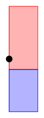
for a viewport to be rotated. For example, consider the image below,
which shows a device (grey rectangle) with a rotated viewport (white
rectangle). The dashed line represents constant x-values within the
viewport and it is clear
that we cannot convert an x-value within the viewport
on its own to an x-value on the
device; we also need to know a y-value within the viewport
(e.g., the dot within the diagram below) in order to
convert an x/y location within the viewport to an x/y location
on the device.
Because of those differences, it is not possible to add a general-purpose "din" (device inches) unit to 'grid'.
For this particular example, an alternative approach would be to
draw the pie chart and the bar plot ourselves with
direct 'grid' calls,
e.g., grid.polygon and grid.rect,
rather than relying on calls to high-level
'graphics' functions. That would possibly simplify the problem
because we could have greater control over the placement of the
pie and the bar.
However, this would not always be the case.
For example, if we were combining output from a more complex
'graphics' function, such as the
plot.dendrogram function, it would be much harder to
replace the high-level function call with our own direct calls to
'grid' functions.
The scenario considered in this report represents a general
class of graphics problems where we want the convenience
of using someone else's high-level plotting functions combined with the
ability to query and revisit the low-level details of what those
functions drew.
Another possibility to consider is producing the image with something other than R. What makes this sort of customisation possible in R is that there are high-level graphics packages like 'lattice' and 'ggplot2' (plus 'graphics' via 'gridGraphics') for drawing complete plots, but they do their drawing using a lower-level graphics system, 'grid', that records the graphical objects and coordinate systems and provides tools for modifying and querying and revisiting those lower-level details of the complete plot. Two non-R graphics systems that bear some resemblance to this arrangement are, within the TeX world, the PGF/TikZ package (Tantau, 2015) with PGFPLOTS (Feuersanger, 2012) built on top and, within the Javascript world, the D3.js library (Bostock et al., 2011) and plotting systems built on top of it, like C3.js (Tanaka, 2018).
The similarity in the case of D3 lies in the fact that it provides a higher level interface for generating HTML and SVG (and CSS) images, but the image that it produces is pure HTML and SVG (and CSS). This means that it is possible to use low-level DOM (Document Object Model) tools to customise an image that was created by D3. For example, the following javascript code uses the C3.js library (which uses D3.js) to create a simple stacked barplot from a high-level description.
The next javascript code uses low-level DOM tools to determine the location of the bars that the C3.js library drew and adds a black dot on the left edge.
PGF/TikZ is a very powerful and flexible low-level graphics system and
PGFPLOTS provides a high-level interface for producing plots with
PGF/TikZ, but
the result can be manipulated using PGF/TikZ itself.
For example, the following LaTeX code uses PGFPLOTS to draw a simple
stacked barplot (the axis environment and the
\addplot commands), but then adds a black dot using a
low-level PGF/TikZ node, with the location of the node
being calculated by querying the PGFPLOTS system
(/pgfplots/xmin).
In comparison to both cases, 'grid' (plus 'lattice' or 'ggplot2' or 'graphics'/'gridGraphics') is unusual and possibly unique in its explicit support for revisiting coordinate systems and providing transformations between coordinate systems. Also, with 'grid' being in the R world, there are many more tools for data processing and calculations.
This report describes a complex R graphics customisation with the following important features: two 'graphics' based plots are combined together on the same page, then further drawing is added that spans the coordinate systems of both plots.
The solution consists of the following steps:
convert the 'graphics' plots to 'grid' plots using
grid.echo from the 'gridGraphics' package;
use 'grid' functions grid.ls and
grid.grep to determine the names of important
grobs and the names of the viewports that they are drawn within;
navigate down to those viewports and use
grobX, grobY, and a new function
deviceLoc to calculate important locations within each
plot in terms of inches on the graphics device;
navigate back up to the "root" viewport to draw the annotations
that span both plots based on the locations in terms of inches
on the graphics device.
The examples and discussion in this document are mostly relevant
to any recent R version (e.g., anything in the 3.* series).
However, the functions deviceLoc and deviceDim
are only available in the
development version of R (revision r74634),
which will become R version 3.6.0.
This report was generated within a Docker container (see Resources section below).
Murrell, P. (2018). "Extreme Makeover: R Graphics Edition." Technical Report 2018-04, Department of Statistics, The University of Auckland. [ bib ]
This document
by Paul
Murrell is licensed under a Creative
Commons Attribution 4.0 International License.