 |
SQL is a language for creating, configuring, and querying relational databases. It is an open standard that is implemented by all major DBMS software, which means that it provides a consistent way to communicate with a database no matter which DBMS software is used to store or access the data.
Like all languages, there are different versions of SQL. The information in this chapter is consistent with SQL-92.
SQL consists of three components:
In this section, we are only concerned with one particular command within the DML part of SQL: the SELECT command for extracting values from tables within a database.
Section 8.3 includes brief information about some of the other features of SQL.
Everything we do in this section will be a variation on the SELECT command of SQL, which has the following basic form:
This will extract the specified columns from the specified tables but it will only include the rows for which the row_condition is true.
The keywords SELECT, FROM, and WHERE are written in uppercase by convention and the names of the columns and tables will depend on the database that is being queried.
Throughout this section, SQL code examples will be presented after a “prompt”, >, and the result of the SQL code will be displayed below the code.
The goal for contestants in the Data Expo was to summarize the important features of the atmospheric measurements. In this section, we will perform some straightforward explorations of the data in order to demonstrate a variety of simple SQL commands.
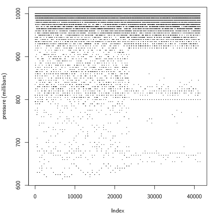
A basic first step in data exploration is just to view the univariate distribution of each measurement variable. The following code extracts all air pressure values from the database using a very simple SQL query that selects all rows from the pressure column of the measure_table.
> SELECT pressure FROM measure_table;
pressure
--------
835.0
810.0
810.0
775.0
795.0
915.0
...
This SELECT command has no restriction on the rows, so the result contains all rows from the table. There are 41,472 ( 24 x 24 x 72) rows in total, so only the first few are shown here. Figure 7.1 shows a plot of all of the pressure values.
|
The resolution of the data is immediately apparent; the pressure is only recorded to the nearest multiple of 5. However, the more striking feature is the change in the spread of the second half of the data. NASA has confirmed that this change is real but unfortunately has not been able to give an explanation for why it occurred.
An entire column of data from the measure_table in the Data Expo database represents measurements of a single variable at all locations for all time periods. One interesting way to “slice” the Data Expo data is to look at the values for a single location over all time periods. For example, how does surface temperature vary over time at a particular location?
The following code shows a slight modification of the previous query to obtain a different column of values, surftemp, and to only return some of the rows from this column. The WHERE clause limits the result to rows for which the location column has the value 1.
> SELECT surftemp
         FROM measure_table
         WHERE location = 1;
surftemp
--------
272.7
282.2
282.2
289.8
293.2
301.4
...
Again, the result is too large to show all values, so only the first few are shown. Figure 7.2 shows a plot of all of the values.
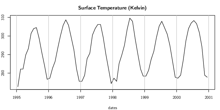 |
The interesting feature here is that we can see a cyclic change in temperature, as we might expect, with the change of seasons.
The order of the rows in a database table is not guaranteed. This means that whenever we extract information from a table, we should be explicit about the order in which we want for the results. This is achieved by specifying an ORDER BY clause in the query. For example, the following SQL command extends the previous one to ensure that the temperatures for location 1 are returned in chronological order.
SELECT surftemp
    FROM measure_table
    WHERE location = 1
    ORDER BY date;
The WHERE clause can use other comparison operators besides equality. As a trivial example, the following code has the same result as the previous example by specifying that we only want rows where the location is less than 2 (the only location value less than two is the value 1).
SELECT surftemp
    FROM measure_table
    WHERE location < 2
    ORDER BY date;
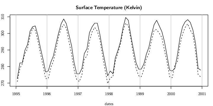
It is also possible to combine several conditions within the WHERE clause, using logical operators AND, to specify conditions that must both be true, and OR, to specify that we want rows where either of two conditions are true. As an example, the following code extracts the surface temperature for two locations. In this example, we include the location and date columns in the result to show that rows from both locations (for the same date) are being included in the result.
> SELECT location, date, surftemp
         FROM measure_table
         WHERE location = 1 OR
               location = 2
         ORDER BY date;
location  date  surftemp
--------  ----  --------
1         1     272.7
2         1     270.9
1         2     282.2
2         2     278.9
1         3     282.2
2         3     281.6
...
Figure 7.3 shows a plot of all of the values, which shows a clear trend of lower temperatures overall for location 2 (the dashed line).
The above query demonstrates that SQL code, even for a single query, can become quite long. This means that we should again apply the concepts from Section 2.4.3 to ensure that our code is tidy and easy to read. The code in this chapter provides many examples of the use of indenting to maintain order within an SQL query.
 |
As well as extracting raw values from a column, it is possible to calculate derived values by combining columns with simple arithmetic operators or by using a function to produce the sum or average of the values in a column.
As a simple example, the following code calculates the average surface temperature value across all locations and across all time points. It crudely represents the average surface temperature of Central America for the years 1995 to 2000.
> SELECT AVG(surftemp) avgstemp
         FROM measure_table;
avgstemp
--------
296.2310
One extra feature to notice about this example SQL query is that it defines a column alias, avgstemp, for the column of averages. The components of this part of the code are shown below.
| keyword: | SELECT AVG(surftemp) avgstemp |
| column name: | SELECT AVG(surftemp) avgstemp |
| column alias: | SELECT AVG(surftemp) avgstemp |
This part of the query specifies that we want to select the average surface temperature value, AVG(surftemp), and that we want to be able to refer to this column by the name avgstemp. This alias can be used within the SQL query, which can make the query easier to type and easier to read, and the alias is also used in the presentation of the result. Column aliases will become more important as we construct more complex queries later in the section.
An SQL function will produce a single overall value for a column of a table, but what is usually more interesting is the value of the function for subgroups within a column, so the use of functions is commonly combined with a GROUP BY clause, which results in a separate summary value computed for subsets of the column.
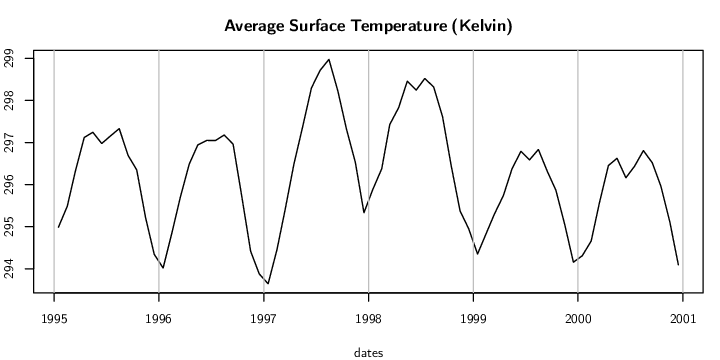
For example, instead of investigating the trend in surface temperature over time for just location 1, we could look at the change in the surface temperature over time averaged across all locations (i.e., the average surface temperature for each month).
The following code performs this query and Figure 7.4 shows a plot of the result. The GROUP BY clause specifies that we want an average surface temperature value for each different value in the date column (i.e., for each month).
> SELECT date, AVG(surftemp) avgstemp
         FROM measure_table
         GROUP BY date
         ORDER BY date;
date avgstemp ---- -------- 1 294.9855 2 295.4869 3 296.3156 4 297.1197 5 297.2447 6 296.9769 ... |
Overall, it appears that 1997 and 1998 were generally warmer years in Central America. This result probably corresponds to the major El Niño event of 1997-1998.
 |
There can be ambiguity whenever we sort or compare text values. A simple example of this issue is deciding whether an upper-case `A' comes before a lower-case `a'. More complex issues arise when comparing text from different languages.
The solution to this ambiguity is to explicitly specify a rule for comparing or sorting text. For example, a case-insensitive rule says that `A' and `a' should be treated as the same character.
In most databases, this sort of rule is called a collation.
Unfortunately, the default collation that is used may differ between database systems, as can the syntax for specifying a collation.
For example, with SQLite, the default is to treat text as case-sensitive, and a case-insensitive ordering can be obtained by adding a COLLATE NOCASE clause to a query.
In MySQL, it may be necessary to specify a collation clause, for example, COLLATE latin1_bin, in order to get case-sensitive sorting and comparisons.
As demonstrated in the previous section, database queries from a single table are quite straightforward. However, most databases consist of more than one table, and most interesting database queries involve extracting information from more than one table. In database terminology, most queries involve some sort of join between two or more tables.
In order to demonstrate the most basic kind of join, we will briefly look at a new example data set.
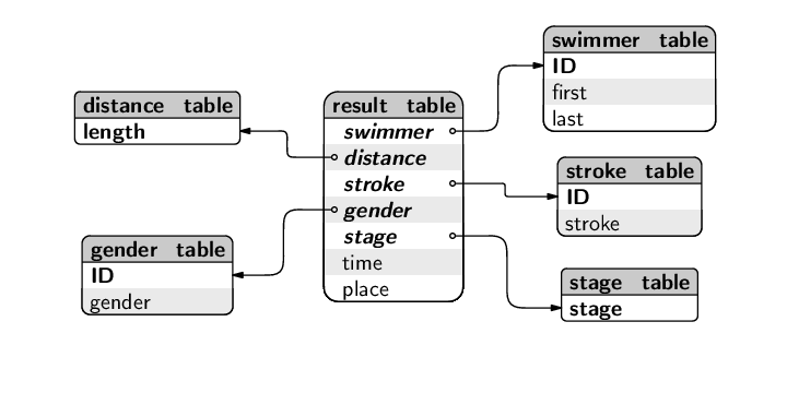
New Zealand sent a team of 18 swimmers to the Melbourne 2006 Commonwealth Games. Information about the swimmers, the events they competed in, and the results of their races are shown in Figure 7.5.
|
first last length stroke gender stage time place ------ ----- ------ ------------ ------ ----- ------ ----- Zoe Baker 50 Breaststroke female heat 31.7 4 Zoe Baker 50 Breaststroke female semi 31.84 5 Zoe Baker 50 Breaststroke female final 31.45 4 Lauren Boyle 200 Freestyle female heat 121.11 8 Lauren Boyle 200 Freestyle female semi 120.9 8 Lauren Boyle 100 Freestyle female heat 56.7 10 Lauren Boyle 100 Freestyle female semi 56.4 9 ... |
These data have been stored in a database with six tables.
The swimmer_table has one row for each swimmer and contains the first and last name of each swimmer. Each swimmer also has a unique numeric identifier.
swimmer_table ( ID [PK], first, last )
There are four tables that define the set of valid events: the distances are 50m, 100m, and 200m; the swim strokes are breaststroke (Br), freestyle (Fr), butterfly (Bu), and backstroke (Ba); the genders are male (M) and female (F); and the possible race stages are heats (heat), semifinals (semi), and finals (final).
distance_table ( length [PK] )
stroke_table ( ID [PK], stroke )
gender_table ( ID [PK], gender )
stage_table ( stage [PK] )
The result_table contains information on the races swum by individual swimmers. Each row specifies a swimmer and the type of race (distance, stroke, gender, and stage). In addition, the swimmer's time and position in the race (place) are recorded.
result_table ( swimmer [PK] [FK swimmer_table.ID],
               distance [PK] [FK distance_table.length],
               stroke [PK] [FK stroke_table.ID],
               gender [PK] [FK gender_table.ID],
               stage [PK] [FK stage_table.stage],
               time, place )
The database design is illustrated in the diagram below.
As an example of the information stored in this database, the following code shows that the swimmer with an ID of 1 is called Zoe Baker. This SQL query, and the next, are not joins, they are just simple one-table queries to show what sort of data is contained in the database.
> SELECT * FROM swimmer_table
         WHERE ID = 1;
ID  first  last
--  -----  -----
1   Zoe    Baker
Notice the use of * in this query to denote that we want all columns from the table in our result.
The following code shows that Zoe Baker swam in three races--a heat,
a semifinal and the final of the women's 50m breaststroke--and she
came ![]() in the final in a time of 31.45 seconds.
in the final in a time of 31.45 seconds.
> SELECT * FROM result_table
         WHERE swimmer = 1;
swimmer distance stroke gender stage time place ------- -------- ------ ------ ----- ----- ----- 1 50 Br F final 31.45 4 1 50 Br F heat 31.7 4 1 50 Br F semi 31.84 5 |
The most basic type of database join, upon which all other types of join are conceptually based, is a cross join. The result of a cross join is the Cartesian product of the rows of one table with the rows of another table. In other words, row 1 of table 1 is paired with each row of table 2, then row 2 of table 1 is paired with each row of table 2, and so on. If the first table has n1 rows and the second table has n2 rows, the result of a cross join is a table with n1 x n2 rows.
The simplest way to create a cross join is simply to perform an SQL query on more than one table. As an example, we will perform a cross join on the distance_table and stroke_table in the swimming database to generate all possible combinations of swimming stroke and event distance. The distance_table has three rows.
> SELECT *
         FROM distance_table;
length ------ 50 100 200 |
The stroke_table has four rows.
> SELECT *
         FROM stroke_table;
ID stroke -- ------------ Br Breaststroke Fr Freestyle Bu Butterfly Ba Backstroke |
A cross join between these tables has 12 rows, including all possible combinations of the rows of the two tables.
> SELECT length, stroke
         FROM distance_table, stroke_table;
length  stroke
------  ------------
50      Breaststroke
50      Freestyle
50      Butterfly
50      Backstroke
100     Breaststroke
100     Freestyle
100     Butterfly
100     Backstroke
200     Breaststroke
200     Freestyle
200     Butterfly
200     Backstroke
A cross join can also be obtained more explicitly using the CROSS JOIN syntax as shown below (the result is exactly the same as for the code above).
SELECT length, stroke
    FROM distance_table CROSS JOIN stroke_table;
We will come back to this data set later in the chapter.
An inner join is the most common way of combining two tables. In this sort of join, only “matching” rows are extracted from two tables. Typically, a foreign key in one table is matched to the primary key in another table.
This is the natural way to combine information from two separate tables.
Conceptually, an inner join is a cross join, but with only the desired rows retained.
In order to demonstrate inner joins, we will return to the Data Expo database (see Section 7.1).
In a previous
example (page ![]() ),
we saw that the surface temperatures from the Data Expo data set
for location 1
were consistently higher than the surface temperatures for location 2.
Why is this?
),
we saw that the surface temperatures from the Data Expo data set
for location 1
were consistently higher than the surface temperatures for location 2.
Why is this?
One obvious possibility is that location 1 is closer to the equator than location 2. To test this hypothesis, we will repeat the earlier query but add information about the latitude and longitude of the two locations.
To do this we need information from two tables. The surface temperatures come from the measure_table and the longitude/latitude information comes from the location_table.
The following code performs an inner join between these two tables, combining rows from the measure_table with rows from the location_table that have the same location ID.
> SELECT longitude, latitude, location, date, surftemp
         FROM measure_table mt, location_table lt
         WHERE location = ID AND
               (location = 1 OR
                location = 2)
         ORDER BY date;
longitude  latitude  location  date  surftemp
---------  --------  --------  ----  --------
-113.75    36.25     1         1     272.7
-111.25    36.25     2         1     270.9
-113.75    36.25     1         2     282.2
-111.25    36.25     2         2     278.9
-113.75    36.25     1         3     282.2
-111.25    36.25     2         3     281.6
...
The result shows that the longitude for location 2 is less negative (less westward) than the longitude for location 1, so the difference between the locations is that location 2 is to the east of location 1 (further inland in the US southwest).
The most important feature of this code is the fact that it obtains information from two tables.
FROM measure_table mt, location_table lt
Another important feature of this code is that it makes use of table aliases. The components of this part of the code are shown below.
| keyword: | FROM measure_table mt, location_table lt |
| table name: | FROM measure_table mt, location_table lt |
| table alias: | FROM measure_table mt, location_table lt |
| table name: | FROM measure_table mt, location_table lt |
| table alias: | FROM measure_table mt, location_table lt |
We have specified that we want information from the measure_table and we have specified that we want to use the alias mt to refer to this table within the code of this query. Similarly, we have specified that the alias lt can be used instead of the full name location_table within the code of this query. This makes it easier to type the code and can also make it easier to read the code.
A third important feature of this code is that, unlike the cross join from the previous section, in this join we have specified that the rows from one table must match up with rows from the other table. In most inner joins, this means specifying that a foreign key from one table matches the primary key in the other table, which is precisely what has been done in this case; the location column from the measure_table is a foreign key that references the ID column from the location_table.
WHERE location = ID
The result is that we get the longitude and latitude information combined with the surface temperature information for the same location.
The WHERE clause in this query also demonstrates the combination of three separate conditions: there is a condition matching the foreign key of the measure_table to the primary key of the location_table, plus there are two conditions that limit our attention to just two values of the location column. The use of parentheses is important to control the order in which the conditions are combined.
Another way to specify the join in the previous query uses a different syntax that places all of the information about the join in the FROM clause of the query. The following code produces exactly the same result as before but uses the key words INNER JOIN between the tables that are being joined and follows that with a specification of the columns to match ON. Notice how the WHERE clause is much simpler in this case.
SELECT longitude, latitude, location, date, surftemp
    FROM measure_table mt
        INNER JOIN location_table lt
            ON mt.location = lt.ID
    WHERE location = 1 OR
          location = 2
    ORDER BY date;
This idea of joining tables extends to more than two tables. In order to demonstrate this, we will now consider a major summary of temperature values: what is the average temperature per year, across all locations on land (above sea level)?
In order to answer this question, we need to know the temperatures from the measure_table, the elevation from the location_table, and the years from the date_table. In other words, we need to combine all three tables.
This situation is one reason for using the INNER JOIN syntax shown above, because it naturally extends to joining more than two tables and results in a clearer and tidier query. The following code performs the desired query (see Figure 7.6).
> SELECT year, AVG(surftemp) avgstemp
         FROM measure_table mt
              INNER JOIN location_table lt
                  ON mt.location = lt.ID
              INNER JOIN date_table dt
                  ON mt.date = dt.ID
         WHERE elevation > 0
         GROUP BY year;
year  avgstemp
----  --------
1995  295.3807
1996  295.0065
1997  295.3839
1998  296.4164
1999  295.2584
2000  295.3150
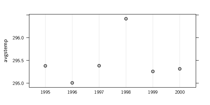 |
The result in Figure 7.6 shows only 1998 as warmer than other years, which suggests that the higher temperatures for 1997 that we saw in Figure 7.4 were due to higher temperatures over water.
There is another important new feature of SQL syntax in the code for this query, which occurs within the part of the code that specifies which columns the inner join should match ON. This part of the code is reproduced below.
ON mt.location = lt.ID
This code demonstrates that, within an SQL query, a column may be specified using a combination of the table name and the column name, rather than just using the column name. In this case, we have defined an alias for each table, so we can use the table alias rather than the complete table name. The components of this part of the code are shown below.
| table name (alias): | ON mt.location = lt.ID |
| column name: | ON mt. location = lt.ID |
| table name (alias): | ON mt.location = lt.ID |
| column name: | ON mt.location = lt. ID |
This syntax is important when joining several tables because the same column name can be used in two different tables. This is the case in the above example; both the location_table and the date_table have a column called ID. This syntax allows us to specify exactly which ID column we mean.
It is possible to use an SQL query within another SQL query, in which case the nested query is called a subquery.
As a simple example, consider the problem of extracting the date at which the lowest surface temperature occurred. It is simple enough to determine the minimum surface temperature.
> SELECT MIN(surftemp) min FROM measure_table; min ----- 266.0 |
In order to determine the date, we need to find the row of the measurement table that matches this minimum value. We can do this using a subquery as shown below.
> SELECT date, surftemp stemp
         FROM measure_table
         WHERE surftemp = ( SELECT MIN(surftemp)
                                FROM measure_table );
date stemp ---- ----- 36 266.0 |
The query that calculates the minimum surface temperature is inserted within parentheses as a subquery within the WHERE clause. The outer query returns only the rows of the measure_table where the surface temperature is equal to the minimum.
This subquery can be part of a more complex query. For example, the following code also performs a join so that we can see the real date on which this minimum temperature occurred.
> SELECT year, month, surftemp stemp
         FROM measure_table mt
             INNER JOIN date_table dt
                 ON mt.date = dt.ID
         WHERE surftemp = ( SELECT MIN(surftemp)
                                FROM measure_table );
year month stemp ---- -------- ----- 1997 December 266.0 |
Another type of table join is the outer join, which differs from an inner join by including additional rows in the result.
In order to demonstrate this sort of join, we will return to the Commonwealth swimming example.
The results of New Zealand's swimmers at the 2006 Commonwealth Games in Melbourne are stored in a database consisting of six tables: a table of information about each swimmer; separate tables for the distance of a swim event, the type of swim stroke, the gender of the swimmers in an event, and the stage of the event (heat, semifinal, or final); plus a table of results for each swimmer in different events.
In Section 7.2.6 we saw how to generate all possible combinations of distance and stroke in the swimming database using a cross join between the distance_table and the stroke_table. There are three possible distances and four different strokes, so the cross join produced 12 different combinations.
We will now take that cross join and combine it with the table of race results using an inner join.
Our goal is to summarize the result of all races for a particular combination of distance and stroke by calculating the average time from such races. The following code performs this inner join, with the results ordered from fastest event on average to slowest event on average.
The cross join produces all possible combinations of distance and stroke and the result table is then joined to that, making sure that the results match up with the correct distance and stroke.
> SELECT dt.length length,
            st.stroke stroke,
            AVG(time) avg
         FROM distance_table dt
             CROSS JOIN stroke_table st
             INNER JOIN result_table rt
                 ON dt.length = rt.distance AND
                    st.ID = rt.stroke
         GROUP BY dt.length, st.stroke
         ORDER BY avg;
length  stroke        avg
------  ------------  -----
50      Freestyle     26.16
50      Butterfly     26.40
50      Backstroke    28.04
50      Breaststroke  31.29
100     Butterfly     56.65
100     Freestyle     57.10
100     Backstroke    60.55
100     Breaststroke  66.07
200     Freestyle     118.6
200     Butterfly     119.0
200     Backstroke    129.7
The result suggests that freestyle and butterfly events tend to be faster on average than breaststroke and backstroke events.
However, the feature of the result that we need to focus on for the current purpose is that this result has only 11 rows.
What has happened to the remaining combination of distance and stroke? The answer is that, for inner joins, a row is not included in the result if either of the two columns being matched in the ON clause has the value NULL.
In this case, one row from the cross join, which produced all possible combinations of distance and stroke, has been dropped from the result because this combination does not appear in the result_table; no New Zealand swimmer competed in the 200m breaststroke.
This feature of inner joins is not always desirable and can produce misleading results, which is why an outer join is sometimes necessary. The idea of an outer join is to retain in the final result rows where one or another of the columns being matched has a NULL value.
The following code repeats the previous query, but instead of using INNER JOIN, it uses LEFT JOIN to perform a left outer join so that all distance/stroke combinations are reported, even though there is no average time information available for one of the combinations. The result now includes all possible combinations of distance and stroke, with a NULL value where there is no matching avg value from the result_table.
> SELECT dt.length length,
            st.stroke stroke,
            AVG(time) avg
         FROM distance_table dt
             CROSS JOIN stroke_table st
             LEFT JOIN result_table rt
                 ON dt.length = rt.distance AND
                    st.ID = rt.stroke
         GROUP BY dt.length, st.stroke
         ORDER BY avg;
length  stroke        avg
------  ------------  -----
200     Breaststroke  NULL
50      Freestyle     26.16
50      Butterfly     26.40
50      Backstroke    28.04
50      Breaststroke  31.29
100     Butterfly     56.65
100     Freestyle     57.10
100     Backstroke    60.55
100     Breaststroke  66.07
200     Freestyle     118.6
200     Butterfly     119.0
200     Backstroke    129.7
The use of LEFT JOIN in this example is significant because it means that all rows from the original cross join are retained even if there is no matching row in the result_table.
It is also possible to use RIGHT JOIN to perform a right outer join instead. In that case, all rows of the result_table (the table on the right of the join) would have been retained.
In this case, the result of a right outer join would be the same as using INNER JOIN because all rows of the result_table have a match in the cross join. This is not surprising because it is equivalent to saying that all swimming results came from events that are a subset of all possible combinations of event stroke and event distance.
It is also possible to use FULL JOIN to perform a full outer join, in which case all rows from tables on both sides of the join are retained in the final result.
It is useful to remember that database joins always begin, at least conceptually, with a Cartesian product of the rows of the tables being joined. The different sorts of database joins are all just different subsets of a cross join. This makes it possible to answer questions that, at first sight, may not appear to be database queries.
For example, it is possible to join a table with itself in what is called a self join, which produces all possible combinations of the rows of a table. This sort of join can be used to answer questions that require comparing a column within a table to itself or to other columns within the same table. The following case study provides an example.
Consider the following question: did the temperature at location 1 for January 1995 (date 1) occur at any other locations and times?
This question requires a comparison of one row of the temperature column in the measure_table with the other rows in that column. The code below performs the query using a self join.
> SELECT mt1.temperature temp1, mt2.temperature temp2,
            mt2.location loc, mt2.date date
         FROM measure_table mt1, measure_table mt2
         WHERE mt1.temperature = mt2.temperature AND
               mt1.date = 1 AND
               mt1.location = 1;
temp1 temp2 loc date ----- ----- --- ---- 272.1 272.1 1 1 272.1 272.1 498 13 |
To show the dates as real dates and locations as longitudes and latitudes, we can join the result to the date_table as well.
> SELECT mt1.temperature temp1, mt2.temperature temp2,
            lt.longitude long, lt.latitude lat, dt.date date
         FROM measure_table mt1, measure_table mt2
            INNER JOIN date_table dt
                ON mt2.date = dt.ID
            INNER JOIN location_table lt
                ON mt2.location = lt.ID
         WHERE mt1.temperature = mt2.temperature AND
               mt1.date = 1 AND
               mt1.location = 1;
temp1  temp2  long     lat     date
-----  -----  -------  ------  ----------
272.1  272.1  -113.75  36.25   1995-01-16
272.1  272.1  -71.25   -13.75  1996-01-16
The temperature occurred again for January 1996 in a location far to the east and south of location 1.
One major advantage of SQL is that it is implemented by every major DBMS. This means that we can learn a single language and then use it to work with any database.
Not all DBMS software supports all of the SQL standard and most DBMS software has special features that go beyond the SQL standard. However, the basic SQL queries that are described in this chapter should work in any major DBMS.
Another major difference between DBMS software is the user interface. In particular, the commercial systems tend to have complete GUIs while the open-source systems tend to default to a command-line interface. However, even a DBMS with a very sophisticated GUI will have a menu option somewhere that will allow SQL code to be run.
The simplest DBMS for experimenting with SQL is the SQLite system7.1because it is very straightforward to install. This section provides a very brief example SQLite session.
SQLite is run from a command window or shell by typing the name of the program plus the name of the database that we want to work with. For example, at the time of writing, the latest version of SQLite was named sqlite3. We would type the following to work with the dataexpo database.
sqlite3 dataexpo
SQLite then presents a prompt, usually sqlite>. We type SQL code after the prompt and the result of our code is printed out to the screen. For example, a simple SQL query with the dataexpo database is shown below, with the result shown below the code.
sqlite> SELECT * FROM date_table WHERE ID = 1;

1|1995-01-16|January|1995
There are a number of special SQLite commands that control how the SQLite program works. For example, the .mode, .header, and .width commands control how SQLite formats the results of queries. The following example shows the use of these special commands to make the result include column names and to use fixed-width columns for displaying results.
sqlite> .header ON
sqlite> .mode column
sqlite> .width 2 10 7 4
sqlite> SELECT * FROM date_table WHERE ID = 1;

ID  date        month    year
--  ----------  -------  ----
1   1995-01-16  January  1995
The full set of these special SQLite commands can be viewed by typing .help.
To exit the SQLite command line, type .exit.
An SQL query can limit which columns and which rows are returned from a database table.
Information can be combined from two or more database tables using some form of database join: a cross join, an inner join, an outer join, or a self join.
Paul Murrell

This work is licensed under a Creative Commons Attribution-Noncommercial-Share Alike 3.0 New Zealand License.