Subsections

10.3 Functions

This section provides a list of some of the functions that are useful for working with data in R. The descriptions of these functions are very brief and only some of the arguments to each function are mentioned. For a complete description of the function and its arguments, the relevant function help page should be consulted (see Section 10.4).

10.3.1 Session management

This section describes some functions that are useful for querying and controlling the R software environment during an interactive session.

ls()

List the symbols that have had values assigned to them during the current session.

$\usebox{\rmbox}$

Delete one or more symbols (the value that was assigned to the symbol is no longer accessible). The symbols to delete are specified by name or as a list of names.

To delete all symbols in the current session, use rm(list=ls()) (carefully).

options(...)

Set a global option for the R session by specifying a new value with an appropriate argument name in the form optionName=optionValue or query the current setting for an option by specifying "optionName".

Typing options() with no arguments returns a list of all current option settings.

q()

Exit the current R session.

10.3.2 Generating vectors

c(...)

Create a new vector by concatenating or combining the values (or vectors of values) given as arguments. All values must be of the same type (or they will be coerced to the same type).

This function can also be used to concatenate lists.

$\usebox{\seqbox}$

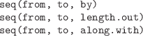
Generate a sequence of numbers from the value from to (not greater than) the value to in steps of by, or for a total of length.out values, or so that the sequence has the same length as along.with.

The function seq_len(n) is faster for producing the sequence from 1 to n and seq_along(x) is faster for producing the sequence from 1 to the number of values in x. These may be useful for producing very long sequences.

The colon operator, :, provides a short-hand syntax for sequences of integer values in steps of 1. The expression from:to is equivalent to seq(from, to).

$\usebox{\repbox}$

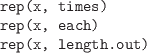
Repeat all values in a vector times times, or each value in the vector each times, or all values in the vector until the total number of values is length.out.

append(x, values, after)

Insert the values into the vector x at the position specified by after.

unlist(x)

Convert a list structure into a vector by concatenating all components of the list. This is especially useful when a function call returns a list where each component is a vector.

rev(x)

Reverse the elements of a vector.

unique(x)

Remove any duplicated values from x.

10.3.3 Numeric functions

sum(..., na.rm=FALSE)

Sum the value of all arguments. If NA values are included, the result is NA (unless na.rm=TRUE).

mean(x)

Calculate the arithmetic mean of the values in x.

$\usebox{\minmaxbox}$

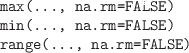
Calculate the minimum, maximum, or range of all values in all arguments.

The functions which.min() and which.max() return the index of the minimum or maximum value within a vector.

diff(x)

Calculate the difference between successive values of x. The result contains one fewer values than there are in x.

$\usebox{\cumbox}$

The cumulative sum or cumulative product of the values in x.

10.3.4 Comparisons

identical(x, y)

Tests whether x and y are equivalent down to the details of their representation in computer memory.

all.equal(target, current, tolerance)

Tests whether target and current differ by only a tiny amount, where “tiny” is defined by tolerance). This is useful for testing whether numeric values are equal.

match(x, table)

Determine the location of each element of x in the set of values in table. The result is a numeric index the same length as x.

The %in% operator is similar (x %in% table), but returns a logical vector the same length as x reporting whether each element of x was found in table.

The pmatch() function performs partial matching (whereas match() is exact).

$\usebox{\isbox}$

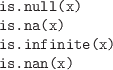
These functions should be used to test for the special values NULL, NA, Inf, and NaN.

$\usebox{\allbox}$

Test whether all or any values in one or more logical vectors are TRUE. The result is a single logical value.

10.3.5 Type coercion

$\usebox{\asbox}$

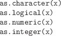
Convert the data structure x to a vector of the appropriate type.

$\usebox{\datebox}$

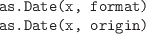
Convert character values or numeric values to Date values.

Character values are converted automatically if they are in ISO 8601 format; otherwise, it may be necessary to describe the date format via the format argument. The help page for the strftime() function describes the syntax for specifying date formats.

When converting numeric values, a reference date must be provided, via the origin argument.

The Sys.Date() function returns today's date as a date value.

The months() function resolves date values just to month names. There are also functions for weekdays() and quarters().

$\usebox{\roundbox}$

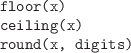
Round a numeric vector, x, to digits decimal places or to an integer value. floor() returns largest integer not greater than x and ceiling() returns smallest integer not less than x.

signif(x, digits)

Round a numeric vector, x, to digits significant digits.

10.3.6 Exploring data structures

$\usebox{\attrbox}$

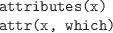
Extract a list of all attributes, or just the attributes named in the character vector which, from the data structure x.

$\usebox{\namebox}$

Extract the names attribute from a vector or list, or the row names or column names from a two-dimensional data structure, or the list of names for all dimensions of an array.

summary(object)

Produces a summary of object. The information displayed will depend on the class of object.

length(x)

The number of elements in a vector, or the number of components in a list. Also works for data frames and matrices, though the result may be less intuitive; it gives the number of columns for a data frame and the total number of values in a matrix.

$\usebox{\dimbox}$

The dimensions of a matrix, array, or data frame. nrow() and ncol() are specifically for two-dimensional data structures, but dim() will also work for higher-dimensional structures.

$\usebox{\headbox}$

Return just the first or last n elements of a data structure; the first elements of a vector, the first few rows of a data frame, and so on.

class(x)

Return the class of the data structure x.

str(object)

Display a summarized, low-level view of a data structure. Typically, the output is less pretty and more detailed than the output from summary().

10.3.7 Subsetting

Subsetting is generally performed via the square bracket operator, [ (e.g., candyCounts[1:4]). In general, the result is of the same class as the original data structure that is being subsetted. The subset may be a numeric vector, a character vector (names), or a logical vector (the same length as the original data structure).

When subsetting data structures with more than one dimension--e.g., data frames, matrices, or arrays--the subset may be several vectors, separated by commas (e.g., candy[1:4, 4]).

The double square bracket operator, [[, selects only one component of a data structure. This is typically used to extract a component from a list.

subset(x, subset, select): Extract the rows of the data frame x that satisfy the condition in subset and the columns that are named in select.

An important special case of subsetting for statistical data sets is the issue of removing missing values from a data set. The function na.omit() can be used to remove all rows containing missing values from a data frame.

10.3.8 Data import/export

R provides general functions for working with the file system.

$\usebox{\wdbox}$

Get the current working directory or set it to dir. This is where R will look for files (or start looking for files).

list.files(path, pattern)

List the names of files in the directory given by path, filtering results with the specified pattern (a regular expression).

For Linux users who are used to using filename globs with the ls shell command, this use of regular expressions for filename patterns can cause confusion. Such users may find the glob2rx() function helpful.

The complete names of the files, including the path, can be obtained by specifying full.names=TRUE. Given a full filename, consisting of a path and a filename, basename() strips off the path to leave just the filename, and dirname() strips off the filename to leave just the path.

file.path(...)

Given the names of nested directories, combine them using an appropriate separator to form a path.

file.choose()

Interactively select a file (on Windows, using a dialog box interface).

$\usebox{\filebox}$

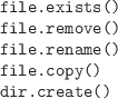
These functions perform the standard file manager tasks of copying, deleting, and renaming files and creating new directories.

There are a number of functions for reading data from external text files into R.

readLines(con)

Read the text file specified by the filename or path given by con. The file specification can also be a URL. The result is a character vector with one element for each line in the file.

read.table(file, header=FALSE, skip=0, sep="")

Read the text file specified by the character value in file, treating each line of text as a case in a data set that contains values for each variable in the data set, with values separated by the character value in sep. Ignore the first skip lines in the file. If header is TRUE, treat the first line of the file as variable names.

The default behavior is to treat columns that contain only numbers as numeric and to treat everything else as a factor. The arguments as.is and stringsAsFactors can be used to produce character variables rather than factors. The colClasses argument provides further control over the type of each column.

This function can be slow on large files because of the work it does to determine the type of values in each column.

The result of this function is a data frame.

read.fwf(file, widths)

Read a text file in fixed-width format. The name of the file is specified by file and widths is a numeric vector specifying the width of each column of values.

The result is a data frame.

read.csv(file)

A front end for read.table() with default argument settings designed for reading a text file in CSV format.

The result is a data frame.

read.delim(file)

A front end for read.table() with default argument settings designed for reading a tab-delimited text file.

The result is a data frame.

scan(file, what)

Read data from a text file and produce a vector of values. The type of the value provided for the argument what determines how the values in the text file are interpreted. If this argument is a list, then the result is a list of vectors, each of a type corresponding to the relevant component of what.

This function is more flexible and faster than read.table() and its kin, but the result may be less convenient to work with.

In most cases, these functions that read a data set from a text file produce a data frame as the result. The functions automatically determine the data type for each column of the data frame, treating anything that is not a number as a factor, but arguments are provided to explicitly specify the data types for columns. Where names of columns are provided in the text file, these functions may modify the names so that they do not cause syntax problems, but again arguments are provided to stop these modifications from happening.

The XML package provides functions for reading and manipulating XML documents.

The package foreign contains various functions for reading data from external files in the various binary formats of popular statistical programs. Other popular scientific binary formats can also be read using an appropriate package, e.g., ncdf for the netCDF format.

Most of the functions for reading files have a corresponding function to write the relevant format.

writeLines(text, con)

Write a character vector to a text file. Each element of the character vector is written as a separate line in the file.

write.table(x, file, sep=" ")

Write a data frame to a text file using a delimited format. The sep argument allows control over the delimiter.

The function write.csv() provides useful defaults for producing files in CSV format.

sink(file)

Redirect R output to a text file. Instead of displaying output on the screen, output is saved into a file. The redirection is terminated by calling sink() with no arguments.

The function capture.output() provides a convenient way to redirect output for a single R expression.

Most of these functions read or write an entire file worth of data in one go. For large data sets, it is also possible to read or write data in smaller pieces. The functions file() and close() allow a file to be held open while reading or writing. Functions that read from files typically have an argument that specifies a number of lines or bytes of information to read, and functions that write to files typically provide an append argument to ensure that previous content is not overwritten.

One important case not mentioned so far is the export and import of data in an R-specific format, which is useful for sharing data between colleagues who all use R.

save(..., file): Save the symbols named in ... (and their values), in an R-specific format, to the specified file.
load(file): Load R symbols (and their values) from the specified file (that has been created by a previous call to save()).
dump(list, file): Write out a text representation of the R data structures named in the character vector list. The data structures can be recreated in R by calling source() on the file.
source(file): Parse and evaluate the R code in file. This can be used to read data from a file created by dump() or much more generally to run any R code that has been stored in a file.

10.3.9 Transformations

transform(data, ...)

Redefine existing columns within a data frame and append new columns to a data frame.

Each argument in ... is of the form columnName=columnValue.

ifelse(test, yes, no)

The test argument is a logical vector. This function creates a new vector consisting of the values in the vector yes when the corresponding element of test is TRUE and the values in no when test is FALSE.

The switch() function is similar, but allows for more than two values in test.

cut(x, breaks)

Transform the continuous vector x into a factor. The breaks argument can be an integer that specifies how many different levels to break x into, or it can be a vector of interval boundaries that are used to cut x into different levels.

An additional labels argument allows labels to be specified for the levels of the new factor.

10.3.10 Sorting

sort(x, decreasing=FALSE): Sort the elements of a vector. Character values are sorted alphabetically (which may depend on the locale or language setting).
order(..., decreasing=FALSE): Determine an ordering based on the elements of one or more vectors. In the simple case of a single vector, sort(x) is equivalent to x[order(x)]. The advantage of this function is that it can be used to reorder more than just a single vector, plus it can produce an ordering from more than one vector; it can break ties in one variable using the values from another variable.

10.3.11 Tables of counts

table(...)

Generate table of counts for one or more factors. The result is a "table" data structure, with as many dimensions as there are arguments.

The margin.table() function reduces a table to marginal totals, prop.table() converts table counts to proportions of marginal totals, and addmargins() adds margin totals to an existing table.

xtabs(formula, data)

Similar to table() except factors to cross-tabulate are expressed in a formula. Symbols in the formula will be searched for in the data frame given by the data argument.

ftable(...)

Similar to table() except that the result is always a two-dimensional "ftable" data structure, no matter how many factors are used. This makes for a more readable display.

10.3.12 Aggregation

aggregate(x, by, FUN): Call the function FUN for each subset of x defined by the grouping factors in the list by. It is possible to apply the function to multiple variables (x can be a data frame) and it is possible to group by multiple factors (the list by can have more than one component). The result is a data frame. The names used in the by list are used for the relevant columns in the result. If x is a data frame, then the names of the variables in the data frame are used for the relevant columns in the result.

10.3.13 The “apply” functions

apply(X, MARGIN, FUN, ...)

Call a function on each row or each column of a data frame or matrix. The function FUN is called for each row of the matrix X, if MARGIN=1; if MARGIN=2, the function is called for each column of X. All other arguments are passed as arguments to FUN.

The data structure that is returned depends on the value returned by FUN. In the simplest case, where FUN returns a single value, the result is a vector with one value per row (or column) of the original matrix X.

sweep(x, MARGIN, STATS, FUN="-")

If MARGIN=1, for row i of x, subtract element i of STATS. For example, subtract row averages from all rows.

More generally, call the function FUN with row i of x as the first argument and element i of STATS as the second argument.

If MARGIN=2, call FUN for each column of x rather than for each row.

tapply(X, INDEX, FUN, ...)

Call a function once for each subset of the vector X, where the subsets correspond to unique values of the factor INDEX. The INDEX argument can be a list of factors, in which case the subsets are unique combinations of the levels of these factors.

The result depends on how many factors are given in INDEX. For the simple case where there is only one factor and FUN returns a single value, the result is a vector.

lapply(X, FUN, ...)

Call the function FUN once for each component of the list X. The result is a list. Additional arguments are passed on to each call to FUN.

sapply(X, FUN, ...)

Similar to lapply(), but will simplify the result to a vector if possible (e.g., if all components of X are vectors and FUN returns a single value).

mapply(FUN, ..., MoreArgs)

A “multivariate” apply. Similar to lapply(), but will call the function FUN on the first element of each of the supplied arguments, then on the second element of each argument, and so on. MoreArgs is a list of arguments to pass to each call to FUN.

rapply(object, f)

A “recursive” apply. Calls the function f on each component of the list object, but if a component is itself a list, then f is called on each component of that list as well, and so on.

10.3.14 Merging

rbind(...)

Create a new data frame by combining two or more data frames that have the same columns. The result is the union of the rows of the original data frames. This function also works for matrices.

cbind(...)

Create a new data frame by combining two or more data frames that have the same number of rows. The result is the union of the columns of the original data frames. This function also works for matrices.

merge(x, y)

Create a new data frame by combining two data frames in a database join operation. The two data frames will usually have different columns, though they will typically share at least one column, which is used to match the rows. Additional arguments allow the matching column to be specified explicitly.

The default join is an inner join on columns that x and y have in common. Additional arguments allow for the equivalent of inner joins and outer joins.

10.3.15 Splitting

split(x, f): Split a vector or data frame, x, into a list of smaller vectors or data frames. The factor f is used to determine which elements of the original vector or which rows of the original matrix end up in each subset.
unsplit(value, f): Combine a list of vectors into a single vector. The factor f determines the order in which the elements of the vectors are combined.
This function can also be used to combine a list of data frames into a single data frame (as long as the data frames have the same number of columns); in this case, f determines the order in which the rows of the data frames are combined.

10.3.16 Reshaping

stack(x)

Stack the existing columns of data frame x together into a single column and add a new column that identifies which original column each value came from.

aperm(a, perm)

Reorder the dimensions of an array. The perm argument specifies the order of the dimensions.

The special case of transposing a matrix is provided by the t() function.

Functions from the reshape package:

$\usebox{\meltbox}$

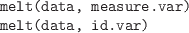
Convert the data, typically a data frame, into “long” form, where there is a row for every measurement or “dependent” value. The measure.var argument gives the names or numeric indices of the variables that contain measurements. All other variables are treated as labels characterizing the measurements (typically factors). Alternatively, the id.var argument specifies the label variables and all others are treated as measurements.

In the resulting data frame, there is a new, single column of measurements with the name value and an additional variable of identifying labels, named variable.

cast(data, formula)

Given data in a long form, i.e., produced by melt(), restructure the data according to the given formula. In the new arrangement, variables mentioned on the left-hand side of the formula vary across rows and variables mentioned on the right-hand side vary across columns.

In a simple repeated-measures scenario consisting of measurements at two time points, the data may consist of a variable of subject IDs plus two variables containing measurements at the two time points.

> library(reshape) > wide <- data.frame(ID=1:3, T1=rnorm(3), T2=sample(100:200, 3)) > wide

ID T1 T2 1 1 -0.5148497 145 2 2 -2.3372321 143 3 3 2.0103460 158

If we melt the data, we produce a data frame with a column named ID, a column named variable with values T1 or T2, and a column named value, containing all of the measurements.

> long <- melt(wide, id.var=c("ID"), measure.var=c("T1", "T2")) > long

ID variable value 1 1 T1 -0.5148497 2 2 T1 -2.3372321 3 3 T1 2.0103460 4 1 T2 145.0000000 5 2 T2 143.0000000 6 3 T2 158.0000000

This form can be recast back to the original wide form as follows.

> cast(long, ID ~ variable)

ID T1 T2 1 1 -0.5148497 145 2 2 -2.3372321 143 3 3 2.0103460 158

The function recast() combines a melt and cast in a single operation.

10.3.17 Text processing

nchar(x)

Count the number of characters in each element of the character vector x. The result is a numeric vector the same length as x.

grep(pattern, x)

Search for the regular expression pattern in the character vector x. The result is a numeric vector identifying which elements of x matched the pattern. If there are no matches, the result has length zero.

The function agrep() allows for approximate matching.

regexpr(pattern, text)

Similar to grep() except that the result is a numeric vector containing the character location of the match within each element of text (-1 if there is no match). The result also has an attribute, match.length, containing the length of the match.

gregexpr(pattern, text)

Similar to regexpr(), except that the result is the locations (and lengths) of all matches within each piece of text. The result is a list.

gsub(pattern, replacement, x)

Search for the regular expression pattern in the character vector x and replace all matches with the character value in replacement. The result is a vector containing the modified text.

The g stands for “global” so all matches are replaced; there is a sub() function that just replaces the first match.

The functions toupper() and tolower() convert character values to all uppercase or all lowercase.

substr(x, start, stop)

For each character value in x, return a subset of the text consisting of the characters at positions start through stop, inclusive. The first character is at position 1.

The function substring() works very similarly, with the extra convenience that the end character defaults to the end of the text.

More specialized text subsetting is provided by the strtim() function, which removes characters from the end of text to enforce a maximum length, and abbreviate(), which reduces text to a given length by removing characters in such a way that each piece of text remains unique.

strsplit(x, split)

For each character value in x, break the text into separate character values, using split as the delimiter. The result is a list, with one character vector component for each element of the original vector x.

paste(..., sep, collapse)

Combine text, placing the character value sep in between. The result is a character vector the same length as the longest of the arguments, so shorter arguments are recycled. If the collapse argument is not NULL, the result vector is then collapsed to a single character value, with the text collapse placed in between each element of the result.

10.3.18 Data display

print(x)

This function generates most of the output that we see on the screen. The important thing to note is that this function is generic, so the output will depend on the class of x. For different classes there are also different arguments to control the way the output is formatted. For example, there is a digits argument that controls the number of significant digits that are printed for numeric values, and there is a quote argument that controls whether double-quotes are printed around character values.

format(x)

The usefulness of this function is to produce a character representation of a data structure where all values have a similar format; for example, all numeric values are formatted to have the same number of characters in total.

sprintf(fmt, ...)

Generates a character vector using the template given by fmt. This is a character value with special codes embedded. Each special code provides a placeholder for values supplied as further arguments to the sprintf() function and the special code controls the formatting of the values. The help page for this function contains a description of the special codes and their meanings.

The usefulness of this function is to obtain fine control over formatting that is not available in print() or format().

strwrap(x, width)

Break long pieces of text, by inserting newlines, so that each line is less than the given width.

cat(..., sep=" ", fill=FALSE)

Displays the values in ... on screen. This function converts its arguments to character vectors if necessary and performs no additional formatting of the text it is given.

The fill argument can be used to control when to start a new line of output, and the sep argument specifies text to place between arguments.

10.3.19 Debugging

The functions from the previous section are useful to display intermediate results from within a loop or function.

debug(fun): Following a call to this function, the function fun will be run one expression at a time, rather than all at once. After each expression, the values of symbols used within the function can be explored by typing the symbol name. Typing `n' (or just hitting Enter) runs the next expression; `c' runs all remaining expressions; and `Q' quits from the function.

Paul Murrell

This work is licensed under a Creative Commons Attribution-Noncommercial-Share Alike 3.0 New Zealand License.