We now have some knowledge of R syntax--what R expressions look like. Before we can start to learn some specific R expressions for particular data processing tasks, we first need to spend some time looking at how information is stored in computer memory.
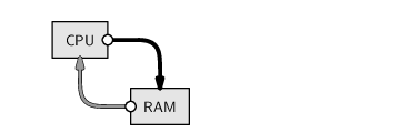
When we are writing code in a programming language, we work most of the time with RAM, combining and restructuring data values to produce new values in RAM.
In Chapter 5, we looked at a number of different data storage formats.
In that discussion, we were dealing with long-term, persistent storage of information on mass storage computer memory.
Although, in this chapter, we will be working in RAM rather than with mass storage, we have exactly the same issues that we had in Chapter 5 of how to represent data values in computer memory. The computer memory in RAM is a series of 0's and 1's, just like the computer memory used to store files in mass storage. In order to work with data values, we need to get those values into RAM in some format.
At the basic level of representing a single number or a single piece of text, the solution is the same as it was in Chapter 5. Everything is represented as a pattern of bits, using various numbers of bytes for different sorts of values. In R, in an English locale, and on a 32-bit operating system, a single character usually takes up one byte, an integer takes four bytes, and a real number 8 bytes. Data values are stored in different ways depending on the data type--whether the values are numbers or text.
Although we do not often encounter the details of the memory representation, except when we need a rough estimate of how much RAM a data set might require, it is important to keep in mind what sort of data type we are working with because the computer code that we write will produce different results for different data types. For example, we can only calculate an average if we are dealing with values that have been stored as numbers, not if the values have been stored as text.
Another important issue is how collections of values are stored in memory. The tasks that we will consider will typically involve working with an entire data set, or an entire variable from a data set, rather than just a single value, so we need to have a way to represent several related values in memory.
This is similar to the problem of deciding on a storage format for a data set, as we discussed in Chapter 5. However, rather than talking about different file formats, in this chapter we will talk about different data structures for storing a collection of data values in RAM. In this section, we will learn about the most common data structures in R.
Throughout this entire chapter, it will be important to always keep clear in our minds what data type we are working with and what sort of data structure are we working with.
Every individual data value has a data type that tells us what sort of value it is. The most common data types are numbers, which R calls numeric values, and text, which R calls character values.
We will meet some other data types as we progress through this section.
We will look at five basic data structures that are available in R.
|
|
|
|
|
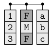
A two-dimensional collection of values that all have the same type.
The values are arranged in rows and columns.
|

|
|
A collection of vectors that all have the same length.
This is like a matrix, except that each column can contain a different
data type.
|
|
|
Starting with the next section, we will use a simple case study to explore the memory representation options available to us. We will also look at some of the functions that are used to create different data structures.
Table 9.1 shows the results of counting how many different sorts of candy there are in a bag of candy. The candies are categorized by their shape (round, oval, or long), their shade (light or dark), and whether they are plain or have a pattern.
In this example, we have information in a table that we can see (on a printed page or on a computer screen) and we want to enter this information into RAM by typing the values on the computer keyboard. We will look at how to write R code to store the information as data structures within RAM.
| Shape | Pattern | Shade | Count |
| round | pattern | light | 2 |
| oval | pattern | light | 0 |
| long | pattern | light | 3 |
| round | plain | light | 1 |
| oval | plain | light | 3 |
| long | plain | light | 2 |
| round | pattern | dark | 9 |
| oval | pattern | dark | 0 |
| long | pattern | dark | 2 |
| round | plain | dark | 1 |
| oval | plain | dark | 11 |
| long | plain | dark | 2 |
We will start by entering the first column of values from Table 9.1--the different shapes of candy. This will demonstrate the c() function for storing data as vectors.
> shapes <- c("round", "oval", "long",
               "round", "oval", "long",
               "round", "oval", "long",
               "round", "oval", "long")
> shapes
 [1] "round" "oval"  "long"  "round" "oval"  "long"  "round"
 [8] "oval"  "long"  "round" "oval"  "long"
|
The information in the first column consists of text, so each individual value is entered as a character value (within quotes), and the overall result is a character vector.
The result has been assigned to the symbol shapes so that we can use this character vector again later.
The second and third columns from Table 9.1 can be stored as character vectors in a similar manner.
> patterns <- c("pattern", "pattern", "pattern",
                 "plain", "plain", "plain",
                 "pattern", "pattern", "pattern",
                 "plain", "plain", "plain")
> patterns
 [1] "pattern" "pattern" "pattern" "plain"   "plain"
 [6] "plain"   "pattern" "pattern" "pattern" "plain"
[11] "plain"   "plain"
|
> shades <- c("light", "light", "light",
               "light", "light", "light",
               "dark", "dark", "dark",
               "dark", "dark", "dark")
> shades
 [1] "light" "light" "light" "light" "light" "light" "dark"
 [8] "dark"  "dark"  "dark"  "dark"  "dark"
|
The c() function also works with numeric values. In the following code, we create a numeric vector to store the fourth column of Table 9.1.
> counts <- c(2, 0, 3, 1, 3, 2, 9, 0, 2, 1, 11, 2)
> counts
[1] 2 0 3 1 3 2 9 0 2 1 11 2
|
We now have the information from Table 9.1 stored as four vectors in RAM.
The previous example demonstrated the c() function for concatenating values together to create a vector. In this section, we will look at some other functions that create vectors.
When data values have a regular pattern, the function rep() is extremely useful (rep is short for “repeat”). For example, column 1 of Table 9.1 has a simple pattern: the set of three possible shapes is repeated four times. The following code generates the shapes vector again, but this time using rep().
> shapes <- rep(c("round", "oval", "long"), 4)
> shapes
 [1] "round" "oval"  "long"  "round" "oval"  "long"  "round"
 [8] "oval"  "long"  "round" "oval"  "long"
|
The first argument to rep() is the vector of values to repeat and the second argument says how many times to repeat the vector. The result is the original vector of 3 values repeated 4 times, producing a final vector with 12 values.
It becomes easier to keep track of what sort of data structure we are dealing with once we become familiar with the way that R displays the different types of data structures. With vectors, R displays an index inside square brackets at the start of each line of output, followed by the values, which are formatted so that they each take up the same amount of space (similar to a fixed-width file format). The previous result had room to display up to seven values on each row, so the second row of output starts with the eighth value (hence the [8] at the start of the line). All of the values have double-quotes around them to signal that these are all character values (i.e., this is a character vector).
As another example of the use of rep(), the following code generates a data structure containing the values in column 2 of Table 9.1.
> patterns <- rep(c("pattern", "plain"), each=3, length=12)
> patterns
 [1] "pattern" "pattern" "pattern" "plain"   "plain"
 [6] "plain"   "pattern" "pattern" "pattern" "plain"
[11] "plain"   "plain"
|
This example demonstrates two other arguments to rep(). The each argument says that each individual element of the original vector should be repeated 3 times. The length argument says that the final result should be a vector of length 12 (without that, the 2 original values would only be repeated 3 times each to produce a vector of 6 values; try it and see!).
To complete the set of variables in the candy data set, the following code generates the shade information from column 3 of Table 9.1.
> shades <- rep(c("light", "dark"), each=6)
> shades
 [1] "light" "light" "light" "light" "light" "light" "dark"
 [8] "dark"  "dark"  "dark"  "dark"  "dark"
|
The rep() function also works for generating numeric vectors; another important function for generating regular patterns of numeric values is the seq() function (seq is short for “sequence”). For example, a numeric vector containing the first 10 positive integers can be created with the following code.
> seq(1, 10)
[1] 1 2 3 4 5 6 7 8 9 10
|
The first argument to seq() specifies the number to start at and the second argument specifies the number to finish at.
There is also a by argument to allow steps in the sequence greater than one, as shown by the following code.
> seq(1, 10, by=3)
[1] 1 4 7 10
|
For integer sequences in steps of 1, a short-hand equivalent is available using the special colon operator, :. For example, we could also have generated the first 10 positive integers with the code below.
> 1:10
[1] 1 2 3 4 5 6 7 8 9 10
|
Going back to the candy data, now that we have Table 9.1 stored as four vectors, we can begin to ask some questions about these data. This will allow us to show that when we perform a calculation with a vector of values, the result is often a new vector of values.
As an example, we will look at how to determine which types of candy did not appear in our bag of candy; in other words, we want to find the values in the counts vector that are equal to zero. The following code performs this calculation using a comparison.
> counts == 0
 [1] FALSE  TRUE FALSE FALSE FALSE FALSE FALSE  TRUE FALSE
[10] FALSE FALSE FALSE
|
This result is interesting for three reasons. The first point is that the result of comparing two numbers for equality is a logical value: either TRUE or FALSE. Logical values are another of the basic data types in R. This result above is a logical vector containing only TRUE or FALSE values.
The second point is that we are starting with a numeric vector, counts, which contains 12 values, and we end up with a new vector that also has 12 values. In general, operations on vectors produce vectors as the result, so a very common way of generating new vectors is to do something with an existing vector.
The third point is that the 12 values in counts are being compared to a single numeric value, 0. The effect is to compare each of the 12 values separately against 0 and return 12 answers. This happens a lot in R when two vectors of different lengths are used. Section 9.6.1 discusses this idea of “recycling” shorter vectors further.
A factor is a basic data structure in R that is ideal for storing categorical data.
For example, consider the shapes vector that we created previously. This was just a character vector recording the text "round" for counts of round candies, "oval" for counts of oval candies, and "long" for counts of long candies.
This is not the ideal way to store this information because it does not acknowledge that elements containing the same text, e.g., "round", really are the same value. A character vector can contain any text at all, so there are no data integrity constraints. The information would be represented better using a factor.
The following code creates the candy shape information as a factor:
> shapesFactor <- factor(shapes,
                          levels=c("round", "oval", "long"))
> shapesFactor
 [1] round oval  long  round oval  long  round oval  long
[10] round oval  long
Levels: round oval long
|
The first argument to the factor() function is the set of data values. We have also specified the set of valid values for the factor via the levels argument.
This is a better representation of the data because every value in the factor shapesFactor is now guaranteed to be one of the valid levels of the factor.
Factors are displayed in a similar way to vectors, but with additional information displayed about the levels of the factor.
A vector in R contains values that are all of the same type. Vectors correspond to a single variable in a data set.
Most data sets consist of more than just one variable, so to store a complete data set we need a different data structure. In R, several variables can be stored together in an object called a data frame.
We will now build a data frame to contain all four variables in the candy data set (i.e., all of the information in Table 9.1).
The function data.frame() creates a data frame object from a set of vectors. For example, the following code generates a data frame from the variables that we have previously created, shapes, patterns, shades, and counts.
> candy <- data.frame(shapes, patterns, shades, counts)
> candy
   shapes patterns shades counts
1   round  pattern  light      2
2    oval  pattern  light      0
3    long  pattern  light      3
4   round    plain  light      1
5    oval    plain  light      3
6    long    plain  light      2
7   round  pattern   dark      9
8    oval  pattern   dark      0
9    long  pattern   dark      2
10  round    plain   dark      1
11   oval    plain   dark     11
12   long    plain   dark      2
|
We now have a data structure that contains the entire data set. This is a significant improvement over having four separate vectors because it properly represents the fact that the first value in each vector corresponds to information about the same type of candy.
An important feature of data frames is the fact that each column within a data frame can contain a different data type. For example, in the candy data frame, the first three columns contain text and the last column is numeric. However, all columns of a data frame must have the same length.
Data frames are displayed in a tabular layout, with column names above and row numbers to the left.
Another detail to notice about the way that data frames are displayed is that the text values in the first three columns do not have double-quotes around them (compare this with the display of text in character vectors in Section 9.4.2). Although character values must always be surrounded by double-quotes when we write code, they are not always displayed with double-quotes.
Vectors, factors, and data frames are the typical data structures that we create to represent our data values in computer memory. However, several other basic data structures are also important because when we call a function, the result could be any sort of data structure. We need to understand and be able to work with a variety of data structures.
As an example, consider the result of the following code:
> dimnames(candy)
[[1]]
 [1] "1"  "2"  "3"  "4"  "5"  "6"  "7"  "8"  "9"  "10" "11"
[12] "12"

[[2]]
[1] "shapes"   "patterns" "shades"   "counts"
|
The dimnames() function extracts the column names and the row names from the candy data frame; these are the values that are displayed above and to the left of the data frame (see the example in the previous section). There are 4 columns and 12 rows, so the dimnames() function has to return two character vectors that have different lengths. A data frame can contain two vectors, but the vectors cannot have different lengths; the only way the dimnames() function can return these values is as a list.
In this case, we have a list with two components. The first component is a character vector containing the 12 row names and the second component is another character vector containing the 4 column names.
Notice the way that lists are displayed. The first component of the list starts with the component index, [[1]], followed by the contents of this component, which is a character vector containing the names of the rows from the data frame.
[[1]]
 [1] "1"  "2"  "3"  "4"  "5"  "6"  "7"  "8"  "9"  "10" "11"
[12] "12"
The second component of the list starts with the component index [[2]], followed by the contents of this component, which is also a character vector, this time the column names.
[[2]]
[1] "shapes"   "patterns" "shades"   "counts"
The list() function can be used to create a list explicitly. Like the c() function, list() takes any number of arguments; if the arguments are named, those names are used for the components of the list.
In the following code, we generate a list similar to the previous one, containing the row and column names from the candy data frame.
> list(rownames=rownames(candy),
        colnames=colnames(candy))
$rownames
 [1] "1"  "2"  "3"  "4"  "5"  "6"  "7"  "8"  "9"  "10" "11"
[12] "12"

$colnames
[1] "shapes"   "patterns" "shades"   "counts"
|
The difference is that, instead of calling dimnames() to get the entire list, we have called rownames() to get the row names as a character vector, colnames() to get the column names as another character vector, and then list() to combine the two character vectors into a list. The advantage is that we have been able to provide names for the components of the list. These names are evident in how the list is displayed on the screen.
A list is a very flexible data structure. It can have any number of components, each of which can be any data structure of any length or size. A simple example is a data-frame-like structure where each column can have a different length, but much more complex structures are also possible. For example, it is possible for a component of a list to be another list.
Anyone who has worked with a computer should be familiar with the idea of a list containing another list because a directory or folder of files has this sort of structure: a folder contains multiple files of different kinds and sizes and a folder can contain other folders, which can contain more files or even more folders, and so on. Lists allow for this kind of hierarchical structure.
Another sort of data structure in R, which lies in between vectors and data frames, is the matrix. This is a two-dimensional structure (like a data frame), but one where all values are of the same type (like a vector).
As for lists, it is useful to know how to work with matrices because many R functions either return a matrix as their result or take a matrix as an argument.
A matrix can be created directly using the matrix() function. The following code creates a matrix from 6 values, with 3 columns and two rows; the values are used column-first.
> matrix(1:6, ncol=3)
     [,1] [,2] [,3]
[1,]    1    3    5
[2,]    2    4    6
|
The array data structure extends the idea of a matrix to more than two dimensions. For example, a three-dimensional array corresponds to a data cube.
The array() function can be used to create an array. In the following code, a two-by-two-by-two, three-dimensional array is created.
> array(1:8, dim=c(2, 2, 2))
, , 1

     [,1] [,2]
[1,]    1    3
[2,]    2    4

, , 2

     [,1] [,2]
[1,]    5    7
[2,]    6    8
|
Although we are not generally concerned with the bit-level or byte-level details of how data values are stored by R in RAM, we do need to be aware of one of the issues that was raised in Section 5.3.1.
In that section, we discussed the fact that there are limits to the precision with which numeric values can be represented in computer memory. This is true of numeric values stored in RAM just as it was for numeric values stored on some form of mass storage.
As a simple demonstration, consider the following condition.
> 0.3 - 0.2 == 0.1
[1] FALSE
|
That apparently incorrect result is occurring because it is not actually possible to store an apparently simple value like 0.1 with absolute precision in computer memory (using a binary representation). The stored value is very, very close to 0.1, but it is not exact. In the condition above, the bit-level representations of the two values being compared are not identical, so the values, in computer memory, are not strictly equal.
Comparisons between real values must be performed with care and tests for equality between real values are not considered to be meaningful. The function all.equal() is useful for determining whether two real values are (approximately) equivalent.
Another issue is the precision to which numbers are displayed. Consider the following simple arithmetic expression.
> 1/3
[1] 0.3333333
|
The answer, to full precision, never ends, but R has only shown seven significant digits. There is a limit to how many decimal places R could display because of the limits of representing numeric values in memory, but there is also a global option that controls (approximately) how many digits that R will display.
The following code uses the options() function to specify that R should display more significant digits.
> options(digits=16)
> 1/3
[1] 0.3333333333333333
|
The code below sets the option back to its default value.
> options(digits=7)
|
A factor is one-dimensional and every element must be one of a fixed set of values, called the levels of the factor.
A matrix is a two-dimensional data structure and all of its elements are of the same type.
A data frame is two-dimensional and different columns may contain different data types, though all values within a column must be of the same data type and all columns must have the same length.
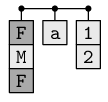
A list is a hierarchical data structure and each component of a list may be any type of data structure whatsoever.
Paul Murrell

This work is licensed under a Creative Commons Attribution-Noncommercial-Share Alike 3.0 New Zealand License.