Now that we know some basic R functions that allow us to enter data values and we have a basic idea of how data values are represented in RAM, we are in a position to start working with the data values.
One of the most basic ways that we can manipulate data structures is to subset them--select a smaller portion from a larger data structure. This is analogous to performing a query on a database.
For example, we might want to answer the question: “what sort of candy was the most common in the bag of candy?” The following code produces the answer to this question using R's subsetting capabilities.
> candy[candy$counts == max(candy$counts), ]
   shapes patterns shades counts
11   oval    plain   dark     11
|
R has very powerful mechanisms for subsetting. In this section, we will outline the basic format of these operations and many more examples will be demonstrated as we progress through the rest of the chapter.
We will start with subsetting vectors.
A subset from a vector may be obtained by appending an index within square brackets to the end of a symbol name. As an example, recall the vector of candy counts, called counts.
> counts
[1] 2 0 3 1 3 2 9 0 2 1 11 2
|
We can extract fourth of these counts by specifying the index 4, as shown below.
> counts[4]
[1] 1
|
The components of this expression are shown below:
| symbol: | counts[4] |
| square brackets: | counts [4 ] |
| index: | counts[ 4] |
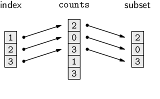
The index can be a vector of any length. For example, the following code produces the first three counts (the number of light-shaded candies with a pattern).
> counts[1:3]
[1] 2 0 3
|
The diagram below illustrates how the values in the index vector are used to select elements from the counts vector to create a subset. Diagrams like this will be used throughout this chapter to help describe different data manipulation techniques; in each case, to save on space, the data values shown in the diagram will not necessarily correspond to the data values being discussed in the surrounding text.
The index does not have to be a contiguous sequence, and it can include repetitions. The following example produces counts for all candies with a pattern. The elements we want are the first three and the seventh, eighth, and ninth. The index is constructed with the following code.
> c(1:3, 7:9)
[1] 1 2 3 7 8 9
|
The subsetting operation is expressed as follows.
> counts[c(1:3, 7:9)]
[1] 2 0 3 9 0 2
|
This is an example of a slightly more complex R expression. It involves a function call, to the c() function, that generates a vector, and this vector is then used as an index to select the corresponding elements from the counts vector.
The components of this expression are shown below:
| symbol: | counts[c(1:3, 7:9)] |
| square brackets: | counts [c(1:3, 7:9) ] |
| index: | counts[ c(1:3, 7:9)] |
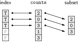
As well as using integers for indices, we can use logical values. For example, a better way to express the idea that we want the counts for all candies with a pattern is to generate a logical vector first, as in the following code.
> hasPattern <- patterns == "pattern"
> hasPattern
 [1]  TRUE  TRUE  TRUE FALSE FALSE FALSE  TRUE  TRUE  TRUE
[10] FALSE FALSE FALSE
|
This logical vector can be used as an index to return all of the counts where hasPattern is TRUE.
> counts[hasPattern]
[1] 2 0 3 9 0 2
|
The diagram below illustrates how an index of logical values selects elements from the complete object where the index value is TRUE.
It would be even better to work with the entire data frame and retain the pattern with the counts, so that we can see that we have the correct result. We will now look at how subsetting works for two-dimensional data structures such as data frames.
A data frame can also be indexed using square brackets, though slightly differently because we have to specify both which rows and which columns we want. The following code extracts the patterns and counts variables, columns 2 and 4, from the data frame for all candies with a pattern:
> candy[hasPattern, c(2, 4)]
  patterns counts
1  pattern      2
2  pattern      0
3  pattern      3
7  pattern      9
8  pattern      0
9  pattern      2
|
The result is still a data frame, just a smaller one.
The components of this expression are shown below:
| symbol: | candy[hasPattern, c(2, 4)] |
| square brackets: | count [hasPattern, c(2, 4) ] |
| row index: | count[ hasPattern, c(2, 4)] |
| comma: | count[hasPattern , c(2, 4)] |
| column index: | count[hasPattern, c(2, 4)] |
An even better way to select this subset is to refer to the appropriate columns by their names. When a data structure has named components, a subset may be selected using those names. For example, the previous subset could also be obtained with the following code.
> candy[hasPattern, c("patterns", "counts")]
  patterns counts
1  pattern      2
2  pattern      0
3  pattern      3
7  pattern      9
8  pattern      0
9  pattern      2
|
The function subset() provides another way to subset a data frame. This function has a subset argument for specifying the rows and a select argument for specifying the columns.
> subset(candy, subset=hasPattern,
          select=c("patterns", "counts"))
  patterns counts
1  pattern      2
2  pattern      0
3  pattern      3
7  pattern      9
8  pattern      0
9  pattern      2
|
When subsetting using square brackets, it is possible to leave the row or column index completely empty. The result is that all rows or all columns, respectively, are returned. For example, the following code extracts all columns for the first three rows of the data frame (the light-shaded candies with a pattern).
> candy[1:3, ]
  shapes patterns shades counts
1  round  pattern  light      2
2   oval  pattern  light      0
3   long  pattern  light      3
|
If a single index is specified when subsetting a data frame with single square brackets, the effect is to extract the appropriate columns of the data frame and all rows are returned.
> candy["counts"]
   counts
1       2
2       0
3       3
4       1
5       3
6       2
7       9
8       0
9       2
10      1
11     11
12      2
|
This result is one that we need to study more closely. This subsetting operation has extracted a single variable from a data frame. However, the result is a data frame containing a single column (i.e., a data set with one variable).
Often what we will require is just the vector representing the values in the variable. This is achieved using a different sort of indexing that uses double square brackets, [[. For example, the following code extracts the first variable from the candy data frame as a vector.
> candy[["counts"]]
[1] 2 0 3 1 3 2 9 0 2 1 11 2
|
The components of this expression are shown below:
| symbol: | candy[["counts"]] |
| double square brackets: | candy [["counts" ]] |
| index: | candy[[ "counts"]] |
Single square bracket subsetting on a data frame is like taking an egg container that contains a dozen eggs and chopping up the container so that we are left with a smaller egg container that contains just a few eggs. Double square bracket subsetting on a data frame is like selecting just one egg from an egg container.
As with single square bracket subsetting, the index used for double square bracket subsetting can also be a number.
> candy[[4]]
[1] 2 0 3 1 3 2 9 0 2 1 11 2
|
However, with double square bracket subsetting, the index must be a single value.
There is also a short-hand equivalent for getting a single variable from a data frame. This involves appending a dollar sign, $, to the symbol, followed by the name of the variable.
> candy$counts
[1] 2 0 3 1 3 2 9 0 2 1 11 2
|
The components of this expression are shown below:
| symbol: | candy$counts |
| dollar sign: | candy $counts |
| variable name: | candy$ counts |
The subsetting syntax can also be used to assign a new value to some portion of a larger data structure. As an example, we will look at replacing the zero values in the counts vector (the counts of candies) with a missing value, NA.
As with extracting subsets, the index can be a numeric vector, a character vector, or a logical vector. In this case, we will first develop an expression that generates a logical vector telling us where the zeroes are.
> counts == 0
 [1] FALSE  TRUE FALSE FALSE FALSE FALSE FALSE  TRUE FALSE
[10] FALSE FALSE FALSE
|
The zeroes are the second and eighth values in the vector.
We can now use this expression as an index to specify which elements of the counts vector we want to modify.
> counts[counts == 0] <- NA
> counts
[1] 2 NA 3 1 3 2 9 NA 2 1 11 2
|
We have replaced the original zero values with NAs.
The following code reverses the process and replaces all NA values with zero. The is.na() function is used to find which values within the counts vector are NAs.
> counts[is.na(counts)] <- 0
|
The case of subsetting a factor deserves special mention because, when we subset a factor, the levels of the factor are not altered. For example, consider the patterns variable in the candy data set.
> candy$patterns
 [1] pattern pattern pattern plain   plain   plain   pattern
 [8] pattern pattern plain   plain   plain
Levels: pattern plain
|
This factor has two levels, pattern and plain. If we subset just the first three values from this factor, the result only contains the value pattern, but there are still two levels.
> candy$patterns[1:3]
[1] pattern pattern pattern
Levels: pattern plain
|
It is possible to force the unused levels to be dropped by specifying drop=TRUE within the square brackets, as shown below.
> subPattern <- candy$patterns[1:3, drop=TRUE]
> subPattern
[1] pattern pattern pattern
Levels: pattern
|
Assigning values to a subset of a factor is also a special case because only the current levels of the factor are allowed. A missing value is generated if the new value is not one of the current factor levels (and a warning is displayed).
For example, in the following code, we attempt to assign a new value to the first element of a factor where the new value is not one of the levels of the factor, so the result is an NA value.
> subPattern[1] <- "swirly"
> subPattern
[1] <NA>    pattern pattern
Levels: pattern
|
[ ], select one or more elements
from a data structure. The result is the same sort of data structure
as the original object, just smaller.
The index within the square brackets can be a numeric vector, a logical vector, or a character vector.
Double square brackets, [[ ]], select a single element
from a data structure. The result is usually a simpler data structure
than the original.
The dollar sign, $, is short-hand for double square brackets.
Paul Murrell

This work is licensed under a Creative Commons Attribution-Noncommercial-Share Alike 3.0 New Zealand License.