This section provides some more details about how R data structures work. The information in this section is a little more advanced, but most of it is still useful for everyday use of R and most of it will be necessary to completely understand some of the R functions that are introduced in later sections.
R allows us to work with vectors of values, rather than with single values, one at a time. This is very useful, but it does raise the issue of what to do when vectors have different lengths.
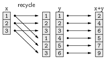
There is a general, but informal, rule in R that, in such cases, the shorter vector is recycled to become the same length as the longer vector. This is easiest to demonstrate via simple arithmetic.
In the following code, a vector of length 3 is added to a vector of length 6.
> c(1, 2, 3) + c(1, 2, 3, 4, 5, 6)
[1] 2 4 6 5 7 9
|
What happens is that the first vector is recycled to make a vector of length 6, and then element-wise addition can occur.
This rule is not necessarily followed in all possible situations, but it is the expected behavior in most cases.
In the case study in Section 9.1, there was a step where we took the text representation of a world population estimate and converted it into a number. This step is repeated below, broken down into a little more detail.
We start with a character vector (containing just one character value).
> popText
[1] "6,617,746,521"
|
We remove the commas from the text, but we still have a character vector.
> popNum <- gsub(",", "", popText)
> popNum
[1] "6617746521"
|
Now, we convert the character vector to a numeric vector.
> pop <- as.numeric(popNum)
> pop
[1] 6617746521
|
The important part is the call to as.numeric(). This is the function that starts with a character value and converts it into a numeric value.
This process is called type coercion and it is important because we need the data in different forms to be able to perform different tasks. In this example, we need the data, which is an estimate of the world population, as a number so that we can subtract it from another, later, estimate of the world population. We cannot do the subtraction on character values.
There are many functions of the form as.type() for deliberately converting between different data structures like this. For example, the function for converting data into a character vector is called as.character().
It is also important to keep in mind that many functions will automatically perform type coercion if we give them an argument in the wrong form. To demonstrate this, we will consider the shapes variable in the candy data frame.
The shapes vector that we created first is a character vector.
> shapes
 [1] "round" "oval"  "long"  "round" "oval"  "long"  "round"
 [8] "oval"  "long"  "round" "oval"  "long"
|
We used this character vector, plus several others, to create the candy data frame, with a call to the data.frame() function.
> candy <- data.frame(shapes, patterns, shades, counts)
|
What do we see if we extract the shapes column from the candy data frame?
> candy$shapes
 [1] round oval  long  round oval  long  round oval  long
[10] round oval  long
Levels: long oval round
|
This is a factor, not a character vector!
How did the original character vector become a factor within the data frame? The data.frame() function automatically performed this type coercion (without telling us!).
This sort of automatic coercion happens a lot in R. Often, it is very convenient, but it is important to be aware that it may be happening, it is important to notice when it happens, and it is important to know how to stop it from happening. In some cases it will be more appropriate to perform type coercion explicitly, with functions such as as.numeric() and as.character(), and in some cases functions will provide arguments that turn the coercion off. For example, the data.frame() function provides a stringsAsFactors argument that controls whether character data are automatically converted to a factor.
As we saw with subsetting factors, performing type coercion requires special care when we are coercing from a factor to another data type.
The correct sequence for coercing a factor is to first coerce it to a character vector and then to coerce the character vector to something else.
In particular, when coercing a factor that has levels consisting entirely of digits, the temptation is to call as.numeric() directly. However, the correct approach is to call as.character() and then as.numeric().
Consider the candy data frame again.
> candy
   shapes patterns shades counts
1   round  pattern  light      2
2    oval  pattern  light      0
3    long  pattern  light      3
4   round    plain  light      1
5    oval    plain  light      3
6    long    plain  light      2
7   round  pattern   dark      9
8    oval  pattern   dark      0
9    long  pattern   dark      2
10  round    plain   dark      1
11   oval    plain   dark     11
12   long    plain   dark      2
|
This data set consists of four variables that record how many candies were counted for each combination of shape, pattern, and shade. These variables are stored in the data frame as three factors and a numeric vector.
The data set also consists of some additional metadata. For example, each variable has a name. How is this information stored as part of the data frame data structure?
The answer is that the column names are stored as attributes of the data frame.
Any data structure in R may have additional information attached to it as an attribute; attributes are like an extra list structure attached to the primary data structure. The diagram below illustrates the idea of a data frame, on the left, with a list of attributes containing row names and column names, on the right.
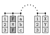
In this case, the data frame has an attribute containing the row names and another attribute containing the column names.
As another example, consider the factor shapesFactor that
we created on page ![]() .
.
> shapesFactor
 [1] round oval  long  round oval  long  round oval  long
[10] round oval  long
Levels: round oval long
|
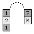
Again, there are the actual data values, plus there is metadata that records the set of valid data values--the levels of the factor. This levels information is stored in an attribute. The diagram below illustrates the idea of a factor, on the left, with a single attribute that contains the valid levels of the factor, on the right.
We do not usually work directly with the attributes of factors or data frames. However, some R functions produce a result that has important information stored in the attributes of a data structure, so it is necessary to be able to work with the attributes of a data structure.
The attributes() function can be used to view all attributes of a data structure. For example, the following code extracts the attributes from the candy data frame (we will talk about the class attribute later).
> attributes(candy)
$names
[1] "shapes"   "patterns" "shades"   "counts"

$row.names
 [1]  1  2  3  4  5  6  7  8  9 10 11 12

$class
[1] "data.frame"
|
This is another result that we should look at very closely. What sort of data structure is it?
This is a list of attributes.
Each component of this list, each attribute of the data frame, has a name; the column names of the candy data frame are in a component of this attribute list called names and the row names of the candy data frame are in a component of this list called row.names.
The attr() function can be used to get just one specific attribute from a data structure. For example, the following code just gets the names attribute from the candy data frame.
> attr(candy, "names")
[1] "shapes" "patterns" "shades" "counts"
|
Because many different data structures have a names attribute, there is a special function, names(), for extracting just that attribute.
> names(candy)
[1] "shapes" "patterns" "shades" "counts"
|
For the case of a data frame, we could also use the colnames() function to get this attribute, and there is a rownames() function for obtaining the row names.
Similarly, there is a special function, levels(), for obtaining the levels of a factor.
> levels(shapesFactor)
[1] "round" "oval" "long"
|
Section 9.9.3 contains an example where it is necessary to directly access the attributes of a data structure.
We can often get some idea of what sort of data structure we are working with by simply viewing how the data values are displayed on screen. However, a more definitive answer can be obtained by calling the class() function.
For example, the data structure that has been assigned to the symbol candy is a data frame.
> class(candy)
[1] "data.frame"
|
The shapes variable within the candy data frame is a factor.
> class(candy$shapes)
[1] "factor"
|
Many R functions return a data structure that is not one of the basic data structures that we have already seen. For example, consider the following code, which generates a table of counts of the number of candies of each different shape (summing across shades and patterns).
We will describe the xtabs() function later in Section 9.8.4. For now, we are just interested in the data structure that is produced by this function.
> shapeCount <- xtabs(counts ~ shapes, data=candy)
> shapeCount
shapes
 long  oval round
    9    14    13
|
What sort of data structure is this? The best way to find out is to use the class() function.
> class(shapeCount)
[1] "xtabs" "table"
|
The result is an "xtabs" data structure, which is a special sort of "table" data structure.
We have not seen either of these data structures before. However, much of what we already know about working with the standard data structures, and some of what we will learn in later sections, will also work with any new class that we encounter.
For example, it is usually possible to subset any class using the standard square bracket syntax. For example, in the following code, we extract the first element from the table.
> shapeCount[1]
long
   9
|
Where appropriate, arithmetic and comparisons will also generally work. In the code below, we are calculating which elements of the table are greater than 10.
> shapeCount > 10
shapes
 long  oval round
FALSE  TRUE  TRUE
|
Furthermore, if necessary, we can often resort to coercing a class to something more standard and familiar. The following code converts the table data structure into a data frame, where the rows of the original table have been converted into columns in the data frame, with appropriate column names automatically provided.
> as.data.frame(shapeCount)
  shapes Freq
1   long    9
2   oval   14
3  round   13
|
In summary, although we will encounter a wide variety of data structures, the standard techniques that we learn in this chapter for working with basic data structures, such as subsetting, will also be useful for working with other classes.
Dates are an important example of a special data structure. Representing dates as just text is convenient for humans to view, but other representations are better for computers to work with.
As an example, we will make use of the Sys.Date() function, which returns the current date.
> today <- Sys.Date()
> today
|
[1] "2008-09-29"
This looks like it is a character vector, but it is not. It is a Date data structure.
> class(today)
[1] "Date"
|
Having a special class for dates means that we can perform tasks with dates,
such as arithmetic
and comparisons, in a meaningful way,
something we could not do if we stored the date as just a character value.
For example, the manuscript for this book was due at the publisher
on September ![]() 2008. The following code
calculates whether the manuscript was late.
The as.Date() function converts a character value,
in this case "2008-09-30", into a date.
2008. The following code
calculates whether the manuscript was late.
The as.Date() function converts a character value,
in this case "2008-09-30", into a date.
> deadline <- as.Date("2008-09-30")
> today > deadline
[1] FALSE
|
The following code calculates how many days remain before the deadline (or how late the manuscript is).
> deadline - today
Time difference of 1 days
|
The Date class stores date values as integer values, representing the
number of days since January ![]() 1970, and
automatically converts the
numbers to a readable text value to display
the dates on the screen.
1970, and
automatically converts the
numbers to a readable text value to display
the dates on the screen.
Another important example of a special class in R is the formula class.
A formula is created by the special tilde operator, ~. Formulas are created to describe relationships using symbols.
We saw an example on page ![]() that looked like
this:
that looked like
this:
> counts ~ shapes
|
The components of this expression are show below:
| left-hand side: | counts ~ shapes |
| tilde operator: | counts ~ shapes |
| right-hand side: | counts ~ shapes |
The result of a formula is just the formula expression itself. A formula only involves the symbol names; any data values that have been assigned to the symbols in the formula are not accessed at all in the creation of the formula.
Each side of a formula can have more than one symbol, with the symbols separated by standard operators such as + and *.
For example, the following call to the xtabs() function combines two symbols on the right-hand side of the formula to produce a two-way table of counts.
> xtabs(counts ~ patterns + shades, data=candy)
         shades
patterns  dark light
  pattern   11     5
  plain     14     6
|
Formulas are mainly used to express statistical models in R, but they are also used in other contexts, such as the xtabs() function shown above and in Section 9.6.4. We will see another use of formulas in Section 9.8.11.
When working with anything but tiny data sets, basic features of the data set cannot be determined by just viewing the data values. This section describes a number of functions that are useful for obtaining useful summary features from a data structure.
The summary() function produces summary information for a data structure. For example, it will provide numerical summary data for each variable in a data frame.
> summary(candy)
   shapes     patterns   shades      counts
 long :4   pattern:6   dark :6   Min.   : 0
 oval :4   plain  :6   light:6   1st Qu.: 1
 round:4                         Median : 2
                                 Mean   : 3
                                 3rd Qu.: 3
                                 Max.   :11
|
The length() function is useful for determining the number of values in a vector or the number of components in a list. Similarly, the dim() function will give the number of rows and columns in a matrix or data frame.
> dim(candy)
[1] 12 4
|
The str() function (short for “structure”) is useful when dealing with large objects because it only shows a sample of the values in each part of the object, although the display is very low-level so it may not always make things clearer.
The following code displays the low-level structure of the candy data frame.
> str(candy)
|
'data.frame':	12 obs. of  4 variables:
 $ shapes  : Factor w/ 3 levels "long","oval",..: 3 2 1 3 ..
 $ patterns: Factor w/ 2 levels "pattern","plain": 1 1 1 2..
 $ shades  : Factor w/ 2 levels "dark","light": 2 2 2 2 2 ..
 $ counts  : num  2 0 3 1 3 2 9 0 2 1 ...
Another function that is useful for inspecting a large object is the head() function. This just shows the first few elements of an object, so we can see the basic structure without seeing all of the values. The code below uses head() to display only the first six rows of the candy data frame.
> head(candy)
  shapes patterns shades counts
1  round  pattern  light      2
2   oval  pattern  light      0
3   long  pattern  light      3
4  round    plain  light      1
5   oval    plain  light      3
6   long    plain  light      2
|
There is also a tail() function for viewing the last few elements of an object.
In Section 9.6.2, we saw that some functions automatically perform type coercion. An example is the paste() function, which combines text values. If we give it a value that is not text, it will automatically coerce it to text. For example, the following code returns a number (the total number of candies in the candy data frame).
> sum(candy$counts)
[1] 36
|
If we use this value as an argument to the paste() function, the number is automatically coerced to a text value to become part of the overall text result.
> paste("There are", sum(candy$counts), "long candies")
[1] "There are 36 long candies"
|
Generic functions are similar in that they will accept many different data structures as arguments. However, instead of forcing the argument to be what the function wants it to be, a generic function adapts itself to the data structure it is given. Generic functions do different things when given different data structures.
An example of a generic function is the summary() function. The result of a call to summary() will depend on what sort of data structure we provide. The summary information for a factor is a table giving how many times each level of the factor appears.
> summary(candy$shapes)
 long  oval round
    4     4     4
|
If we provide a numeric vector, the result is a five-number summary, plus the mean.
> summary(candy$counts)
   Min. 1st Qu.  Median    Mean 3rd Qu.    Max.
      0       1       2       3       3      11
|
Generic functions are another reason why it is easy to work with data in R; a single function will produce a sensible result no matter what data structure we provide.
However, generic functions are also another reason why it is so important to be aware of what data structure we are working with. Without knowing what sort of data we are using, we cannot know what sort of result to expect from a generic function.
Type coercion is the conversion of data values from one data type or data structure to another. This may happen automatically within a function, so care should be taken to make sure that data values returned by a function have the expected data type or data structure.
Any data structure may have attributes, which provide additional information about the data structure. These are in the form of a list of data values that are attached to the main data structure.
All data structures have a class.
Basic data manipulations such as subsetting, arithmetic, and comparisons, should still work even with unfamiliar classes.
Dates and formulas are important examples of special classes.
A generic function is a function that produces a different result depending on the class of its arguments.
Paul Murrell

This work is licensed under a Creative Commons Attribution-Noncommercial-Share Alike 3.0 New Zealand License.