This section describes a number of techniques for rearranging objects in R, particularly larger data structures, such as data frames, matrices, and lists.
Some of these techniques are useful for basic exploration of a data set. For example, we will look at functions for sorting data and for generating tables of counts.
Other techniques will allow us to perform more complex tasks such as restructuring data sets to convert them from one format to another, splitting data structures into smaller pieces, and combining smaller pieces to form larger data structures.
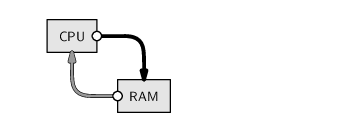
This section is all about starting with a data structure in RAM and calculating new values, or just rearranging the existing values, to generate a new data structure in RAM.
In order to provide a motivation for some of these techniques, we will use the following case study throughout this section.
The New Zealand Ministry of Education provides basic information for all primary and secondary schools in the country.9.2In this case study, we will work with a subset of this information that contains the following variables:
These data have been stored in CSV format in a file called schools.csv (see Figure 9.9).
|
"ID","Name","City","Auth","Dec","Roll" 1015,"Hora Hora School","Whangarei","State",2,318 1052,"Morningside School","Whangarei","State",3,200 1062,"Onerahi School","Whangarei","State",4,455 1092,"Raurimu Avenue School","Whangarei","State",2,86 1130,"Whangarei School","Whangarei","State",4,577 1018,"Hurupaki School","Whangarei","State",8,329 1029,"Kamo Intermediate","Whangarei","State",5,637 1030,"Kamo School","Whangarei","State",5,395 ... |
Using functions from the last section, we can easily read this information into R and store it as a data frame called schools. The as.is argument is used to ensure that the school names are kept as text and are not treated as a factor.
> schools <-
       read.csv(file.path("Schools", "schools.csv"),
                as.is=2)
|
> schools
|
    ID                  Name      City  Auth Dec Roll
1 1015      Hora Hora School Whangarei State   2  318
2 1052    Morningside School Whangarei State   3  200
3 1062        Onerahi School Whangarei State   4  455
4 1092 Raurimu Avenue School Whangarei State   2   86
5 1130      Whangarei School Whangarei State   4  577
6 1018       Hurupaki School Whangarei State   8  329
...
In cases like this, where the data set is much too large to view all at once, we can make use of functions to explore the basic characteristics of the data set. For example, it is useful to know just how large the data set is. The following code tells us the number of rows and columns in the data frame.
> dim(schools)
[1] 2571 6
|
There are 6 variables measured on 2,571 schools.
We will now go on to look at some data manipulation tasks that we could perform on this data set.
A common task in data preparation is to create new variables from an existing data set. As an example, we will generate a new variable that distinguishes between “large” schools and “small” schools.
This new variable will be based on the median school roll. Any school with a roll greater than the median will be “large”.
> rollMed <- median(schools$Roll)
> rollMed
[1] 193
|
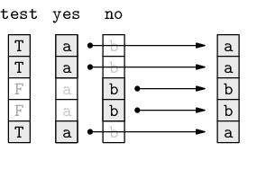
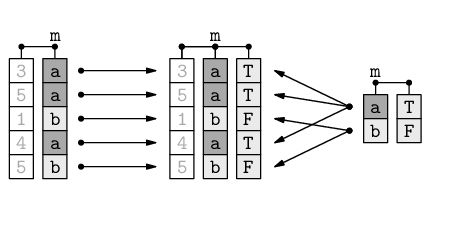
We can use the ifelse() function to generate a character vector recording "large" and "small". The first argument to this function, called test, is a logical vector. The second argument, called yes, provides the result wherever the test argument is TRUE and the third argument, called no, provides the result wherever the test argument is FALSE.
> size <- ifelse(test=schools$Roll > rollMed,
                  yes="large", no="small")
|
> size
|
 [1] "large" "large" "large" "small" "large" "large" "large"
 [8] "large" "large" "large" "large" "large" "small" "large"
...
The diagram below illustrates that the ifelse() function selects elements from the yes argument when the test argument is TRUE and from the no argument when test is FALSE.
We will now add this new variable to the original data frame to maintain the correspondence between the school size labels and the original rolls that they were derived from.
This can be done in several ways. The simplest is to assign a new variable to the data frame, as shown in the following code. The data frame does not have an existing column called Size, so this assignment adds a new column.
> schools$Size <- size
|
> schools
|
    ID                  Name      City  Auth Dec Roll  Size
1 1015      Hora Hora School Whangarei State   2  318 large
2 1052    Morningside School Whangarei State   3  200 large
3 1062        Onerahi School Whangarei State   4  455 large
4 1092 Raurimu Avenue School Whangarei State   2   86 small
5 1130      Whangarei School Whangarei State   4  577 large
6 1018       Hurupaki School Whangarei State   8  329 large
...
Another approach, which gives the same result, is to use the transform() function.
> schools <- transform(schools, Size=size)
|
If we want to remove a variable from a data frame, we can assign the value NULL to the appropriate column.
> schools$size <- NULL
|
Alternatively, we can use subsetting to retain certain columns or leave out certain columns. This approach is better if more than one column needs to be removed. For example, the following code removes the new, seventh column from the data frame.
> schools <- schools[, -7]
|
> schools
|
    ID                  Name      City  Auth Dec Roll
1 1015      Hora Hora School Whangarei State   2  318
2 1052    Morningside School Whangarei State   3  200
3 1062        Onerahi School Whangarei State   4  455
4 1092 Raurimu Avenue School Whangarei State   2   86
5 1130      Whangarei School Whangarei State   4  577
6 1018       Hurupaki School Whangarei State   8  329
...
The previous example converted a numeric variable into two categories, small and large. The more general case is to convert a numeric variable into any number of categories.
For example, rather than just dividing the schools into large and small, we could group the schools into five different size categories. This sort of transformation is possible using the cut() function.
> rollSize <-
       cut(schools$Roll, 5,
           labels=c("tiny", "small", "medium",
                    "large", "huge"))
|
The first argument to this function is the numeric vector to convert. The second argument says that the range of the numeric vector should be broken into five equal-sized intervals. The schools are then categorized according to which interval their roll lies within. The labels argument is used to provide levels for the resulting factor.
Only the first few schools are shown below and they are all tiny; the important point is that the result is a factor with five levels.
> head(rollSize)
[1] tiny tiny tiny tiny tiny tiny
Levels: tiny small medium large huge
|
A better view of the result can be obtained by counting how many schools there are of each size. This is what the following code does; we will see more about functions to create tables of counts in Section 9.8.4.
> table(rollSize)
rollSize
  tiny  small medium  large   huge
  2487     75      8      0      1
|
Another common task that we can perform is to sort a set of values into ascending or descending order.
In R, the function sort() can be used to arrange a vector of values in order, but of more general use is the order() function, which returns the indices of the sorted values.
As an example, the information on New Zealand schools is roughly ordered by region, from North to South in the original file. We might want to order the schools by size instead.
The following code sorts the Roll variable by itself.
> sort(schools$Roll)
|
[1] 5 5 6 6 6 7 7 7 7 8 9 9 9 9 9 9 9 ...
There are clearly some very small schools in New Zealand.
It is also easy to sort in decreasing order, which reveals that the largest school is the largest by quite some margin.
> sort(schools$Roll, decreasing=TRUE)
|
[1] 5546 3022 2613 2588 2476 2452 2417 2315 2266 2170 ...
However, what would be much more useful would be to know which schools these are. That is, we would like to sort not just the school rolls, but the entire schools data frame.
To do this, we use the order() function, as shown in the following code.
> rollOrder <- order(schools$Roll, decreasing=TRUE)
|
> rollOrder
|
[1] 1726 301 376 2307 615 199 467 373 389 241 ...
This result says that, in order to sort the data frame in descending roll order, we should use row 1726 first, then row 301, then row 376, and so on.
These values can be used as indices for subsetting the entire schools data frame, as shown in the following code. Recall that, by only specifying a row index and by leaving the column index blank, we will get all columns of the schools data frame.
> schools[rollOrder, ]
|
      ID                     Name         City  Auth Dec Roll
1726 498    Correspondence School   Wellington State  NA 5546
301   28        Rangitoto College     Auckland State  10 3022
376   78         Avondale College     Auckland State   4 2613
2307 319     Burnside High School Christchurch State   8 2588
615   41         Macleans College     Auckland State  10 2476
199   43       Massey High School     Auckland State   5 2452
467   54         Auckland Grammar     Auckland State  10 2417
373   69 Mt Albert Grammar School     Auckland State   7 2315
389   74       Mt Roskill Grammar     Auckland State   4 2266
...
The largest body of New Zealand school students represents those gaining public education via correspondence (from the governmental base in Wellington), but most of the other large schools are in Auckland, which is the largest city in New Zealand.
The other advantage of using the order() function is that more than one vector of values may be given and any ties in the first vector will be broken by ordering on the second vector. For example, the following code sorts the rows of the schools data frame first by city and then by number of students (in decreasing order). In the case of the City variable, which is a character vector, the order is alphabetic. Again, we are specifying decreasing=TRUE to get descending order.
> schools[order(schools$City, schools$Roll,
                 decreasing=TRUE), ]
|
       ID                      Name      City  Auth Dec Roll
2548  401           Menzies College   Wyndham State   4  356
2549 4054            Wyndham School   Wyndham State   5   94
1611 2742          Woodville School Woodville State   3  147
1630 2640           Papatawa School Woodville State   7   27
2041 3600            Woodend School   Woodend State   9  375
1601  399 Central Southland College    Winton State   7  549
...
The first two schools are both in Wyndham, with the larger school first and the smaller school second, then there are two schools from Woodville, larger first and smaller second, and so on.
Continuing our exploration of the New Zealand schools data set, we might be interested in how many schools are private and how many are state-owned. This is an example where we want to obtain a table of counts for a categorical variable. The function table() may be used for this task.
> authTable <- table(schools$Auth)
|
> authTable
|
           Other          Private            State State Integrated
               1               99             2144              327
This result shows the number of times that each different value occurs in the Auth variable. As expected, most schools are public schools, owned by the state.
As usual, we should take notice of the data structure that this function has returned.
> class(authTable)
[1] "table"
|
This is not one of the basic data structures that we have focused on. However, tables in R behave very much like arrays, so we can use what we already know about working with arrays. For example, we can subset a table just like we subset an array. If we need to, we can also convert a table to an array, or even to a data frame.
As a brief side track, the table of counts above also shows that there is only one school in the category "Other". How do we find that school? One approach is to generate a logical vector and use that to subscript the data frame, as in the following code.
> schools[schools$Auth == "Other", ]
      ID            Name         City  Auth Dec Roll
2315 518 Kingslea School Christchurch Other   1   51
|
It turns out that this school is not state-owned, but still receives its funding from the government because it provides education for students with learning or social difficulties.
Getting back to tables of counts, another question we might ask is how the school decile relates to the school ownership. If we give the table() function more than one argument, it will cross-tabulate the arguments, as the following code demonstrates.
> table(Dec=schools$Dec, Auth=schools$Auth)
    Auth
Dec  Other Private State State Integrated
  1      1       0   259               12
  2      0       0   230               22
  3      0       2   208               35
  4      0       6   219               28
  5      0       2   214               38
  6      0       2   215               34
  7      0       6   188               45
  8      0      11   200               45
  9      0      12   205               37
  10     0      38   205               31
|
Again, the result of this function call is a table data structure. This time it is a two-dimensional table, which is very similar to a two-dimensional array.
In this example, we have provided names for the arguments, Dec and Auth, and these have been used to provide overall labels for each dimension of the table.
This table has one row for each decile and one column for each type of ownership. For example, the third row of the table tells us that there are 2 private schools, 209 state schools, and 35 state integrated schools with a decile of 3.
The most obvious feature of this result is that private schools tend to be in wealthier areas, with higher deciles.
Another function that can be used to generate tables of counts is the xtabs() function. This is very similar to the table() function, except that the factors to cross-tabulate are specified in a formula, rather than as separate arguments.
The two-dimensional table above could also be generated with the following code.
> xtabs( ~ Dec + Auth, data=schools)
|
One advantage of this approach is that the symbols used in the formula are automatically found in the data frame provided in the data argument, so, for example, there is no need to specify the Auth variable as schools$Auth, as we had to do in the previous call to the table() function.
R provides many functions for calculating numeric summaries of data. For example, the min() and max() functions calculate minimum and maximum values for a vector, sum() calculates the sum, and the mean() function calculates the average value. The following code calculates the average value of the number of students enrolled at New Zealand schools.
> mean(schools$Roll)
[1] 295.4737
|
This “grand mean” value is not very interesting by itself. What would be more interesting would be to calculate the average enrolment for different types of schools and compare, for example, state schools and private schools.
We could calculate these values individually, by extracting the relevant subset of the data. For example, the following code extracts just the enrolments for private schools and calculates the mean for those values.
> mean(schools$Roll[schools$Auth == "Private"])
[1] 308.798
|
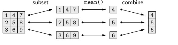
However, a better way to work is to let R determine the subsets and calculate all of the means in one go. The aggregate() function provides one way to perform this sort of task.
The following code uses aggregate() to calculate the average enrolment for New Zealand schools broken down by school ownership.
There are four different values of schools$Auth,
so the result is four averages. We can easily check the answer
for Other schools because there is only one such
school and we saw on page ![]() that this school
has a roll of 51.
that this school
has a roll of 51.
> aggregate(schools["Roll"],
             by=list(Ownership=schools$Auth),
             FUN=mean)
         Ownership     Roll
1            Other  51.0000
2          Private 308.7980
3            State 300.6301
4 State Integrated 258.3792
|
This result shows that the average school size is remarkably similar for all types of school ownership (ignoring the "Other" case because there is only one such school).
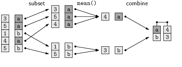
The aggregate() function can take a bit of getting used to, so we will take a closer look at the arguments to this function.
There are three arguments to the aggregate() call. The first argument provides the values that we want to average. In this case, these values are the enrolments for each school. A minor detail is that we have provided a data frame with only one column, the Roll variable, rather than just a vector. It is possible to provide either a vector or a data frame, but the advantage of using a data frame is that the second column in the result has a sensible name.
We could have used schools$Roll, a vector, instead of schools["Roll"], a data frame, but then the right-hand column of the result would have had an uninformative name, x.
The second argument to the aggregate() function is called by and the value must be a list. In this case, there is only one component in the list, the Auth variable, which describes the ownership of each school. This argument is used to generate subsets of the first argument. In this case, we subset the school enrolments into four groups, corresponding to the four different types of school ownership. By providing a name for the list component, Ownership, we control the name of the first column in the result. If we had not done this, then the first column of the result would have had a much less informative name, Group.1.
The third argument to the aggregate() function, called FUN, is the name of a function. This function is called on each subset of the data. In this case, we have specified the mean() function, so we have asked for the average enrolments to be calculated for each different type of school ownership. It is possible to specify any function name here, as long as the function returns only a single value as its result. For example, sum(), min(), and max() are all possible alternatives.
The diagram below provides a conceptual view of how aggregate() works.
In the terminology of data queries in Section 7.2.1, the aggregate() function acts very much like an SQL query with a GROUP BY clause.
Another point to make about the aggregate() function is that the value returned by the function is a data frame. This is convenient because data frames are easy to understand and we have lots of tools for working with data frames.
We will now look at a slightly more complicated use of the aggregate() function. For this example, we will generate a new vector called rich that records whether each school's decile is greater than 5. The following code creates the new vector.
> rich <- schools$Dec > 5
|
> rich
|
[1] FALSE FALSE FALSE FALSE FALSE TRUE FALSE ...
The vector rich provides a crude measure of whether each school is in a wealthy area or not. We will now use this variable in a more complicated call to aggregate().
Because the by argument to aggregate() is a list, it is possible to provide more than one factor. This means that we can produce a result for all possible combinations of two or more factors. In the following code, we provide a list of two factors as the by argument, so the result will be the average enrolments broken down by both the type of school ownership and whether the school is in a wealthy area.
> aggregate(schools["Roll"],
             by=list(Ownership=schools$Auth,
                     Rich=rich),
             FUN=mean)
         Ownership  Rich     Roll
1            Other FALSE  51.0000
2          Private FALSE 151.4000
3            State FALSE 261.7487
4 State Integrated FALSE 183.2370
5          Private  TRUE 402.5362
6            State  TRUE 338.8243
7 State Integrated  TRUE 311.2135
|
The result of the aggregation is again a data frame, but this time there are three columns. The first two columns indicate the different groups and the third gives the average for each group.
The result suggests that, on average, schools in wealthier areas have more students.
One limitation of the aggregate() function is that it only works with functions that return a single value. If we want to calculate, for example, the range of enrolments for each type of school--the minimum and the maximum together--the range() function will perform the calculation for us, but we cannot use range() with aggregate() because it returns two values. Instead, we need to use the by() function.
The following code calculates the range of enrolments for all New Zealand schools, demonstrating that the result is a numeric vector containing two values, 5 and 5546.
> range(schools$Roll)
[1] 5 5546
|
The following code uses the by() function to generate the range of enrolments broken down by school ownership.
> rollRanges <-
       by(schools["Roll"],
          INDICES=list(Ownership=schools$Auth),
          FUN=range)
> rollRanges
Ownership: Other
[1] 51 51
---------------------------------------------
Ownership: Private
[1]    7 1663
---------------------------------------------
Ownership: State
[1]    5 5546
---------------------------------------------
Ownership: State Integrated
[1]   18 1475
|
The arguments to the by() function are very similar to the arguments for aggregate() (with some variation in the argument names) and the effect is also very similar: the first argument is broken into subsets, with one subset for each different value in the second argument, and the third argument provides a function to call on each subset.
However, the result of by() is not a data frame like for aggregate(). It is a very different sort of data structure.
> class(rollRanges)
[1] "by"
|
We have not seen this sort of data structure before, but a by object behaves very much like a list, so we can work with this result just like a list.
The result of the call to by() gives the range of enrolments for each type of school ownership. It suggests that most of the large schools are owned by the state.
In order to motivate some of the remaining sections, here we introduce another, related New Zealand schools data set for us to work with.
The National Certificates of Educational Achievement (NCEA) are used to measure students' learning in New Zealand secondary schools. Students usually attempt to achieve NCEA Level 1 in their third year of secondary schooling, Level 2 in their fourth year, and Level 3 in their fifth and final year of secondary school.
Each year, information on the percentage of students who achieved each NCEA level is reported for all New Zealand secondary schools. In this case study, we will look at NCEA achievement percentages for 2007.
The data are stored in a plain text, colon-delimited format, in a file called NCEA2007.txt. There are four columns of data: the school name, plus the three achievement percentages for the three NCEA levels. Figure 9.10 shows the first few lines of the file.
|
Name:Level1:Level2:Level3
Al-Madinah School:61.5:75:0
Alfriston College:53.9:44.1:0
Ambury Park Centre for Riding Therapy:33.3:20:0
Aorere College:39.5:50.2:30.6
Auckland Girls' Grammar School:71.2:78.9:55.5
Auckland Grammar:22.1:30.8:26.3
Auckland Seventh-Day Adventist H S:50.8:34.8:48.9
Avondale College:57.3:49.8:44.6
Baradene College:89.3:89.7:88.6
...
|
The following code uses the read.table() function to read these data into a data frame called NCEA. We have to specify the colon delimiter via sep=":". Also, because some school names have an apostrophe, we need to specify quote="". Otherwise, the apostrophes are interpreted as the start of a text field. The last two arguments specify that the first line of the file contains the variable names (header=TRUE) and that the first column of school names should be treated as character data (not as a factor).
> NCEA <- read.table(file.path("Schools", "NCEA2007.txt"),
                      sep=":", quote="",
                      header=TRUE, as.is=TRUE)
|
> NCEA
|
                                   Name Level1 Level2 Level3
1                     Al-Madinah School   61.5   75.0    0.0
2                     Alfriston College   53.9   44.1    0.0
3 Ambury Park Centre for Riding Therapy   33.3   20.0    0.0
4                        Aorere College   39.5   50.2   30.6
5        Auckland Girls' Grammar School   71.2   78.9   55.5
6                      Auckland Grammar   22.1   30.8   26.3
7    Auckland Seventh-Day Adventist H S   50.8   34.8   48.9
...
As with the schools data frame, the data set is too large to view all at once, so we will only show a few rows for most examples in the following sections.
The dim() function tells us that, in total, there are 88 schools and 4 variables in this data set. This data set only has Auckland schools.
> dim(NCEA)
[1] 88 4
|
We will now explore this data set in order to demonstrate some more data manipulation techniques.
The NCEA data frame contains three columns of numeric data--the percentage of students achieving NCEA at the three different NCEA levels. Something we could quickly look at is whether the achievement percentages are similar, on average, for each NCEA level.
One way to look at these averages is to extract each column and calculate an average for each column. For example, the following code calculates the average achievement percentage for NCEA Level 1.
> mean(NCEA$Level1)
[1] 62.26705
|
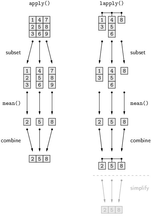
However, as in the aggregation case, there is a smarter way to work, which is to let R extract the columns and calculate a mean for all columns in a single function call. This sort of task is performed by the apply() function.
The following code uses the apply() function to calculate the average achievement percentage for each NCEA level.
> apply(NCEA[2:4], MARGIN=2, FUN=mean)
  Level1   Level2   Level3
62.26705 61.06818 47.97614
|
The result suggests that a slightly lower percentage of students achieve NCEA Level 3 compared to the other NCEA levels.
As with the aggregate() function, the apply() function can take a bit of getting used to, so we will now take a closer look at how the apply() function works.
The apply() function takes three main arguments.
The first argument is expected to be a matrix (or array). In the example above, we have provided the second, third, and fourth columns of the NCEA data frame, i.e., a data frame with three columns, as the first argument. This is an example of a situation that was mentioned back in Section 9.6.2, where a function will silently coerce the value that we supply to another sort of data structure if it needs to.
In this case, the apply() function silently coerces the data frame that we give it into a matrix. The conversion from a data frame to a matrix makes sense in this case because all three columns of the data frame that we supplied are numeric, so the data frame columns convert very naturally and predictably into a matrix (with three columns and 88 rows).
The second argument to apply() specifies how the array should be broken into subsets. The value 1 means split the matrix into separate rows and the value 2 means split the matrix into separate columns. In this case, we have split the matrix into columns; each column represents percentages for one NCEA level.
The third argument specifies a function to call for each subset. In this case, the apply() call says to take each column corresponding to an NCEA level and call the mean() function on each column.
The diagram below provides a conceptual view of how apply() works when MARGIN=1 (apply by rows). Figure 9.11 includes a diagram that illustrates using apply() by columns.
The data structure returned by apply() depends on how many values are returned by the function FUN. In the last example, we used the function mean(), which returns just a single value, so the overall result was a numeric vector, but if FUN returns more than one value, the result will be a matrix.
For example, the following code calls apply() with the range() function to get the range of percentages at each NCEA level. The range() function returns two values for each NCEA level, so the result is a matrix with three columns (one for each NCEA level) and two rows--the minimum and maximum percentage at each level.
> apply(NCEA[2:4], 2, range)
     Level1 Level2 Level3
[1,]    2.8    0.0    0.0
[2,]   97.4   95.7   95.7
|
The basic idea of apply() has similarities with the aggregate() and by() functions that we saw in the previous section. In all of these cases, we are breaking a larger data structure into smaller pieces, calling a function on each of the smaller pieces and then putting the results back together again to create a new data structure.
In the case of aggregate(), we start with a vector or a data frame and we end up with a data frame. The by() function starts with a vector or a data frame and ends up with a list-like object. With apply(), we start with an array and end up with a vector or a matrix.
The lapply() function is another example of this idea. In this case, the starting point is a list. The function breaks the list into its separate components, calls a function on each component, and then combines the results into a new list (see Figure 9.11).
In order to demonstrate the use of lapply(), we will repeat the task we just performed using apply().
The following code calls lapply() to calculate the average percentage of students achieving each NCEA level.
> lapply(NCEA[2:4], FUN=mean)
$Level1
[1] 62.26705

$Level2
[1] 61.06818

$Level3
[1] 47.97614
|
The lapply() function has only two main arguments. The first argument is a list. As with the apply() example, we have supplied a data frame--the second, third, and fourth columns of the NCEA data frame--rather than supplying a list. The lapply() function silently converts the data frame to a list, which is a natural conversion if we treat each variable within the data frame as a component of the list.
The second argument to lapply() is a function to call on each component of the list, and again we have supplied the mean() function.
The result of lapply() is a list data structure. The numeric results, the average percentages for each NCEA level, are exactly the same as they were when we used apply(); all that has changed is that these values are stored in a different sort of data structure.
Like apply(), the lapply() function comfortably handles functions that return more than a single value. For example, the following code calculates the range of percentages for each NCEA level.
> lapply(NCEA[2:4], FUN=range)
$Level1
[1]  2.8 97.4

$Level2
[1]  0.0 95.7

$Level3
[1]  0.0 95.7
|
These results from lapply() are very similar to the previous results from apply(); all that has changed is that the values are stored in a different sort of data structure (a list rather than a matrix).
Whether to use apply() or lapply() will depend on what sort of data structure we are starting with and what we want to do with the result. For example, if we start with a list data structure, then lapply() is the appropriate function to use. However, if we start with a data frame, we can often use either apply() or lapply() and the choice will depend on whether we want the answer as a list or as a matrix.
The sapply() function provides a slight variation on lapply(). This function behaves just like lapply() except that it attempts to simplify the result by returning a simpler data structure than a list, if that is possible. For example, if we use sapply() rather than lapply() for the previous examples, we get a vector and a matrix as the result, rather than lists.
> sapply(NCEA[2:4], mean)
  Level1   Level2   Level3
62.26705 61.06818 47.97614
|
> sapply(NCEA[2:4], range)
     Level1 Level2 Level3
[1,]    2.8    0.0    0.0
[2,]   97.4   95.7   95.7
|
In this section, we will look at the problem of combining data structures.
For simple situations, the functions c(), cbind(), and rbind() are all that we need. For example, consider the two numeric vectors below.
> 1:3
[1] 1 2 3
|
> 4:6
[1] 4 5 6
|
The c() function is useful for combining vectors or lists to make a longer vector or a longer list.
> c(1:3, 4:6)
[1] 1 2 3 4 5 6
|
The functions cbind() and rbind() can be used to combine vectors, matrices, or data frames with similar dimensions. The cbind() function creates a matrix or data frame by combining data structures side-by-side (a “column” bind) and rbind() combines data structures one above the other (a “row” bind).
> cbind(1:3, 4:6)
     [,1] [,2]
[1,]    1    4
[2,]    2    5
[3,]    3    6
|
> rbind(1:3, 4:6)
     [,1] [,2] [,3]
[1,]    1    2    3
[2,]    4    5    6
|
A more difficult problem arises if we want to combine two data structures that do not have the same dimensions.
In this situation, we need to first find out which rows in the two data structures correspond to each other and then combine them.
The diagram below illustrates how two data frames (left and right) can be merged to create a single data frame (middle) by matching up rows based on a common column (labeled m in the diagram).
For example, the two case studies that we have been following in this section provide two data frames that contain information about New Zealand schools. The schools data frame contains information about the location and size of every primary and secondary school in the country, while the NCEA data frame contains information about the NCEA performance of every secondary school.
It would be useful to be able to combine the information from these two data frames. This would allow us to, for example, compare NCEA performance between schools of different sizes.
The merge() function can be used to combine data sets like this.
The following code creates a new data frame, aucklandSchools, that contains information from the schools data frame and from the NCEA data frame for Auckland secondary schools.
> aucklandSchools <- merge(schools, NCEA,
                            by.x="Name", by.y="Name",
                            all.x=FALSE, all.y=FALSE)
|
> aucklandSchools
|
                 Name ID      City    Auth Dec Roll Level1 Level2 Level3
35  Mahurangi College 24 Warkworth   State   8 1095   71.9   66.2   55.9
48      Orewa College 25     Orewa   State   9 1696   75.2   81.0   54.9
32   Long Bay College 27  Auckland   State  10 1611   74.5   84.2   67.2
55  Rangitoto College 28  Auckland   State  10 3022   85.0   81.7   71.6
30     Kristin School 29  Auckland Private  10 1624   93.4   27.8   36.7
19  Glenfield College 30  Auckland   State   7  972   58.4   65.5   45.6
10 Birkenhead College 31  Auckland   State   6  896   59.8   65.7   50.4
...
The first two arguments to the merge() function are the data frames to be merged, in this case, schools and NCEA.
The by.x and by.y arguments specify the names of the variables to use to match the rows from one data frame with the other. In this case, we use the Name variable from each data frame to determine which rows belong with each other.
The all.x argument says that the result should only include schools from the schools data frame that have the same name as a school in the NCEA data frame. The all.y argument means that a school in NCEA must have a match in schools or it is not included in the final result.
By default, merge() will match on any variable names that the two data frames have in common, and it will only include rows in the final result if there is a match between the data frames. In this case, we could have just used the following expression to get the same result:
> merge(schools, NCEA)
|
In the terminology of Section 7.2.4, the merge() function is analogous to a database join.
In relational database terms, by.x and by.y correspond to a primary-key/foreign-key pairing. The all.x and all.y arguments control whether the join is an inner join or an outer join.
The merge() call above roughly corresponds to the following SQL query.
SELECT *
    FROM schools INNER JOIN NCEA
        ON schools.Name = NCEA.Name;
Instead of combining two data frames, it is sometimes useful to break a data frame into several pieces. For example, we might want to perform a separate analysis on the New Zealand schools for each different type of school ownership.
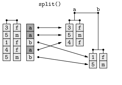
The split() function can be used to break up a data frame into smaller data frames, based on the levels of a factor. The result is a list, with one component for each level of the factor.
The diagram below illustrates how the split() function uses the values within a factor to break a data frame (left) into a list containing two separate data frames (right).
The result is effectively several subsets of the original data frame, but with the subsets all conveniently contained within a single overall data structure (a list), ready for subsequent processing or analysis.
In the following code, the Rolls variable from the schools data frame is broken into four pieces based on the Auth variable.
> schoolRollsByAuth <- split(schools$Roll, schools$Auth)
|
The resulting list, schoolRollsByAuth, has four components, each named after one level of the Auth variable and each containing the number of students enrolled at schools of the appropriate type. The following code uses the str() function that we saw in Section 9.6.7 to show a brief view of the basic structure of this list.
> str(schoolRollsByAuth)
|
List of 4
 $ Other           : int 51
 $ Private         : int [1:99] 255 39 154 73 83 25 95 85 ..
 $ State           : int [1:2144] 318 200 455 86 577 329 6..
 $ State Integrated: int [1:327] 438 26 191 560 151 114 12..
Because the result of split() is a list, it is often used in conjunction with lapply() to perform a task on each component of the resulting list. For example, we can calculate the average roll for each type of school ownership with the following code.
> lapply(schoolRollsByAuth, mean)
$Other
[1] 51

$Private
[1] 308.798

$State
[1] 300.6301

$`State Integrated`
[1] 258.3792
|
This result can be compared to the result we got using the aggregate()
function on page ![]() .
.
For multivariate data sets, where a single individual or case is measured several times, there are two common formats for storing the data.
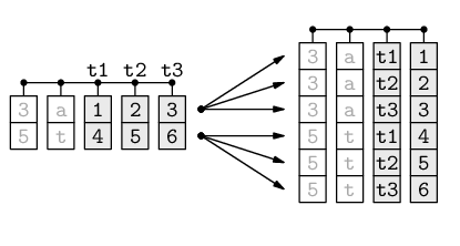
The so-called “wide” format uses a separate variable for each measurement, and the “long” format for a data set has a single observation on each row.
The diagram below illustrates the difference between wide format (on the left), where each row contains multiple measurements (t1, t2, and t3) for a single individual, and long format (on the right), where each row contains a single measurement and there are multiple rows for each individual.
For some data processing tasks, it is useful to have the data in wide format, but for other tasks, the long format is more convenient, so it is useful to be able to convert a data set from one format to the other.
The NCEA data frame that we have been using is in wide format because it has a row for each school and a column for each NCEA level. There is one row per school and three observations on each row.
> NCEA
|
                                   Name Level1 Level2 Level3
1                     Al-Madinah School   61.5   75.0    0.0
2                     Alfriston College   53.9   44.1    0.0
3 Ambury Park Centre for Riding Therapy   33.3   20.0    0.0
4                        Aorere College   39.5   50.2   30.6
5        Auckland Girls' Grammar School   71.2   78.9   55.5
6                      Auckland Grammar   22.1   30.8   26.3
7    Auckland Seventh-Day Adventist H S   50.8   34.8   48.9
...
In the long format of the NCEA data set, each school would have three rows, one for each NCEA level. What this format looks like is shown below. We will go on to show how to obtain this format.
                                   Name variable value
1                     Alfriston College   Level1  53.9
2                     Alfriston College   Level2  44.1
3                     Alfriston College   Level3   0.0
4                     Al-Madinah School   Level1  61.5
5                     Al-Madinah School   Level2  75.0
6                     Al-Madinah School   Level3   0.0
7 Ambury Park Centre for Riding Therapy   Level1  33.3
...
There are several ways to perform the transformation between wide and long formats in R, but we will focus in this section on the reshape package because it provides a wider range of options and a more intuitive set of arguments.
> library("reshape")
|
The two main functions in the reshape package are called melt() and cast(). The melt() function is used to convert a data frame into long format, and the cast() function can then be used to reshape the data into a variety of other forms.
The following code creates the long format version of the NCEA data frame using the melt() function.
> longNCEA <- melt(NCEA, measure.var=2:4)
|
The melt() function typically requires two arguments. The first argument provides the data frame to melt. The second argument is either measure.var to specify which columns of the data frame are observations (reshape calls them “measured” variables) or id.var to specify which columns of the data frame are just values that identify the individual or case (reshape calls these “id” variables).
In the example above, we have specified that the second, third, and fourth columns are observations. The melt() function infers that the first column is therefore an “id” variable. The following code produces an identical result, using the id.var argument instead. In this case, we have specified that the Name variable is an “id” variable and the melt() function will treat all other columns as “measured” variables. This code also demonstrates that columns in the data frame can be specified by name as well as by number.
> longNCEA <- melt(NCEA, id.var="Name")
|
                                   Name variable value
1                     Alfriston College   Level1  53.9
2                     Alfriston College   Level2  44.1
3                     Alfriston College   Level3   0.0
4                     Al-Madinah School   Level1  61.5
5                     Al-Madinah School   Level2  75.0
6                     Al-Madinah School   Level3   0.0
7 Ambury Park Centre for Riding Therapy   Level1  33.3
...
The longNCEA data frame has 264 rows because each of the original 88 schools now occupies three rows.
> dim(longNCEA)
[1] 264 3
|
The original four columns in NCEA have become three columns in longNCEA. The first column in longNCEA is the same as the first column of NCEA, except that all of the values repeat three times.
The second column in longNCEA is called variable and it records which column of NCEA that each row of longNCEA has come from. For example, all values from the original Level1 column in NCEA have the value Level1 in the new variable column in longNCEA.
The third column in longNCEA is called value and this contains all of the data from the Level1, Level2, and Level3 columns of NCEA.
We now turn our attention to the other main function in the reshape package, the cast() function.
As a simple demonstration of the cast() function, we will use it to recreate the original wide format of the NCEA data set. The following code performs this transformation.
> cast(longNCEA, Name ~ variable)
|
                                   Name Level1 Level2 Level3
1                     Alfriston College   53.9   44.1    0.0
2                     Al-Madinah School   61.5   75.0    0.0
3 Ambury Park Centre for Riding Therapy   33.3   20.0    0.0
4                        Aorere College   39.5   50.2   30.6
5        Auckland Girls' Grammar School   71.2   78.9   55.5
6                      Auckland Grammar   22.1   30.8   26.3
7    Auckland Seventh-Day Adventist H S   50.8   34.8   48.9
...
The first argument to cast() is a data frame in long format.
The second argument to cast() is a formula.
Variables on the left-hand side of this formula are used to form the rows of the result and variables on the right-hand side are used to form columns. In the above example, the result contains a row for each different school, based on the Name of the school, and a column for each different NCEA level, where the variable column specifies the NCEA level.
The following code uses a different formula to demonstrate the power that cast() provides for reshaping data. In this case, the data set has been transposed so that each column is now a different school and each row corresponds to one of the NCEA levels.
> tNCEA <- cast(longNCEA, variable ~ Name)
|
> tNCEA
|
  variable Alfriston College Al-Madinah School ...
1   Level1              53.9              61.5 ...
2   Level2              44.1              75.0 ...
3   Level3               0.0               0.0 ...
This data structure has 3 rows and 89 columns: one row for each NCEA level and one column for each school, plus an extra column containing the names of the NCEA levels.
> dim(tNCEA)
[1] 3 89
|
Now that we have seen a number of techniques for manipulating data sets, the next section presents a larger case study that combines several of these techniques to perform a more complex exploration of a data set.
A resident of Baltimore, Maryland, in the United States collected data from his residential gas and electricity power bills over 8 years. The data are in a text file called baltimore.txt and include the start date for the bill, the number of therms of gas used and the amount charged, the number of kilowatt hours of electricity used and the amount charged, the average daily outdoor temperature (as reported on the bill), and the number of days in the billing period. Figure 9.12 shows the first few lines of the data file.
|
start therms gas KWHs elect temp days 10-Jun-98 9 16.84 613 63.80 75 40 20-Jul-98 6 15.29 721 74.21 76 29 18-Aug-98 7 15.73 597 62.22 76 29 16-Sep-98 42 35.81 460 43.98 70 33 19-Oct-98 105 77.28 314 31.45 57 29 17-Nov-98 106 77.01 342 33.86 48 30 17-Dec-98 200 136.66 298 30.08 40 33 19-Jan-99 144 107.28 278 28.37 37 30 18-Feb-99 179 122.80 253 26.21 39 29 ... |
Several events of interest occurred in the household over the time period during which these values were recorded, and one question of interest was to determine whether any of these events had any effect on the energy consumption of the household.
The events were:
The text file containing the energy usage can be read conveniently using the read.table() function, with the header=TRUE argument specified to use the variable names on the first line of the file. We also use as.is=TRUE to keep the dates as text for now.
> utilities <- read.table(file.path("Utilities",
                                     "baltimore.txt"),
                           header=TRUE, as.is=TRUE)
|
> utilities
|
      start therms   gas KWHs elect temp days
1 10-Jun-98      9 16.84  613 63.80   75   40
2 20-Jul-98      6 15.29  721 74.21   76   29
3 18-Aug-98      7 15.73  597 62.22   76   29
4 16-Sep-98     42 35.81  460 43.98   70   33
5 19-Oct-98    105 77.28  314 31.45   57   29
6 17-Nov-98    106 77.01  342 33.86   48   30
...
The first thing we want to do is to convert the first variable into actual dates. This will allow us to perform calculations and comparisons on the date values.
> utilities$start <- as.Date(utilities$start,
                              "%d-%b-%y")
|
> utilities
|
       start therms   gas KWHs elect temp days
1 1998-06-10      9 16.84  613 63.80   75   40
2 1998-07-20      6 15.29  721 74.21   76   29
3 1998-08-18      7 15.73  597 62.22   76   29
4 1998-09-16     42 35.81  460 43.98   70   33
5 1998-10-19    105 77.28  314 31.45   57   29
6 1998-11-17    106 77.01  342 33.86   48   30
...
The next thing that we will do is break the data set into five different time “phases,” using the four significant events as breakpoints; we will be interested in the average daily charges for each of these phases.
To keep things simple, we will just determine the phase based on whether the billing period began before a significant event.
The six critical dates that we will use to categorize each billing period are the start of the first billing period, the dates at which the significant events occurred, and the start of the last billing period.
> breakpoints <- c(min(utilities$start),
                    as.Date(c("1999-07-31", "2004-04-22",
                              "2004-09-01", "2005-12-18")),
                    max(utilities$start))
> breakpoints
[1] "1998-06-10" "1999-07-31" "2004-04-22" "2004-09-01"
[5] "2005-12-18" "2006-08-17"
|
We can use the cut() function to convert the start variable, which contains the billing period start dates, into a phase variable, which is a factor.
> phase <- cut(utilities$start, breakpoints,
                include.lowest=TRUE, labels=FALSE)
> phase
 [1] 1 1 1 1 1 1 1 1 1 1 1 1 1 2 2 2 2 2 2 2 2 2 2 2 2 2 2 2
[29] 2 2 2 2 2 2 2 2 2 2 2 2 2 2 2 2 2 2 2 2 2 2 2 2 2 2 2 2
[57] 2 2 2 2 2 2 2 2 2 2 2 2 3 3 3 3 4 4 4 4 4 5 4 4 4 4 4 4
[85] 4 4 4 4 4 5 5 5 5 5 5 5
|
Each billing period now has a corresponding phase.
One important point to notice about these phase values
is that they are not strictly increasing. In particular,
the ![]() value is a 5 amongst a run of 4s.
This reveals that the billing periods in the original file were
not entered in strictly chronological order.
value is a 5 amongst a run of 4s.
This reveals that the billing periods in the original file were
not entered in strictly chronological order.
Now that we have each billing period assigned to a corresponding phase, we can sum the energy usage and costs for each phase. This is an application of the aggregate() function. The following code subsets the utilities data frame to remove the first column, the billing period start dates, and then sums the values in all of the remaining columns for each different phase.
> phaseSums <- aggregate(utilities[c("therms", "gas", "KWHs",
                                      "elect", "days")],
                          list(phase=phase), sum)
|
> phaseSums
  phase therms     gas  KWHs   elect days
1     1    875  703.27  5883  602.84  406
2     2   5682 5364.23 24173 2269.14 1671
3     3     28   76.89  1605  170.27  124
4     4   1737 2350.63  5872  567.91  483
5     5    577  847.38  3608  448.61  245
|
We can now divide the totals for each phase by the number of days in each phase to obtain an average usage and cost per day for each phase.
> phaseAvgs <- phaseSums[2:5]/phaseSums$days
|
For inspecting these values, it helps if we round the values to two significant figures.
> signif(phaseAvgs, 2)
  therms  gas KWHs elect
1   2.20 1.70   14   1.5
2   3.40 3.20   14   1.4
3   0.23 0.62   13   1.4
4   3.60 4.90   12   1.2
5   2.40 3.50   15   1.8
|
The division step above works because when a data frame is divided by a vector, each variable in the data frame gets divided by the vector. This is not necessarily obvious from the code; a more explicit way to perform the operation is to use the sweep() function, which forces us to explicitly state that, for each row of the data frame (MARGIN=1), we are dividing (FUN="/") by the corresponding value from a vector (STAT=phase$days).
> phaseSweep <- sweep(phaseSums[2:5],
                       MARGIN=1, STAT=phaseSums$days, FUN="/")
|
Looking at the average daily energy values for each phase, the values that stand out are the gas usage and cost during phase 3 (after the first two storm windows were replaced, but before the second set of four storm windows were replaced). The naive interpretation is that the first two storm windows were incredibly effective, but the next four storm windows actually made things worse again!
At first sight this appears strange, but it is easily explained by the fact that phase 3 coincided with summer months, as shown below using the table() function. This code produces a rough count of how many times each month occurred in each phase. The function months() extracts the names of the months from the dates in the start variable; each billing period is assigned to a particular month based on the month that the period started in (which is why this is a rough count).
> table(months(utilities$start), phase)[month.name, ]
           phase
            1 2 3 4 5
  January   1 5 0 1 1
  February  1 5 0 1 1
  March     0 5 0 1 1
  April     1 5 0 1 1
  May       1 3 1 1 1
  June      2 4 1 1 1
  July      2 4 1 1 1
  August    1 5 1 1 1
  September 1 5 0 2 0
  October   1 5 0 2 0
  November  1 4 0 2 0
  December  1 5 0 2 0
|
Subsetting the resulting table by the predefined symbol month.name just rearranges the order of the rows of the table; this ensures that the months are reported in calendar order rather than alphabetical order.
We would expect the gas usage (for heating) to be a lot lower during summer. This is confirmed by (roughly) calculating the daily average usage and cost for each month.
Again we must take care to get the answer in calendar order; this time we do that by creating a factor that is based on converting the start of each billing period into a month, with the order of the levels of this factor explicitly set to be month.name.
> billingMonths <- factor(months(utilities$start),
                           levels=month.name)
|
We then use aggregate() to sum the usage, costs, and days for the billing periods, grouped by this billingMonths factor.
> months <-
       aggregate(utilities[c("therms", "gas", "KWHs",
                             "elect", "days")],
                 list(month=billingMonths),
                 sum)
|
Finally, we divide the usage and cost totals by the number of days in the billing periods. So that we can easily comprehend the results, we cbind() the month names on to the averages and round the averages using signif().
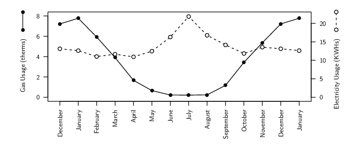
> cbind(month=months$month,
         signif(months[c("therms", "gas",
                         "KWHs", "elect")]/months$days,
                2))
       month therms  gas KWHs elect
1    January   7.80 7.50   13   1.2
2   February   5.90 5.90   11   1.0
3      March   3.90 4.00   12   1.1
4      April   1.70 1.90   11   1.0
5        May   0.65 0.99   12   1.3
6       June   0.22 0.57   16   1.8
7       July   0.21 0.59   22   2.3
8     August   0.23 0.60   17   1.8
9  September   1.20 1.30   14   1.3
10   October   3.40 3.50   12   1.1
11  November   5.40 5.50   14   1.2
12  December   7.20 7.10   13   1.2
|
These results are presented graphically in Figure 9.13.
This example has demonstrated a number of data manipulation techniques in a more realistic setting. The simple averages that we have calculated serve to show that any attempt to determine whether the significant events led to a significant change in energy consumption and cost for this household is clearly going to require careful analysis.
 |
Aggregation involves producing a summary value for each group in a data set.
An “apply” operation calculates a summary value for each variable in a data frame, or for each row or column of a matrix, or for each component of a list.
Data frames can be merged just like tables can be joined in a database. They can also be split apart.
Reshaping involves transforming a data set from a row-per-subject, “wide”, format to a row-per-observation, “long”, format (among other things).
Paul Murrell

This work is licensed under a Creative Commons Attribution-Noncommercial-Share Alike 3.0 New Zealand License.