9.7 Data import/export

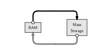
Almost all of the examples so far have used data that are typed explicitly as R expressions. In practice, data usually reside in one or more files of various formats and in some form of mass storage. This section looks at R functions that can be used to read data into R from such external files.

We will look at functions that deal with all of the different data storage options that were discussed in Chapter 5: plain text files, XML documents, binary files, spreadsheets, and databases.

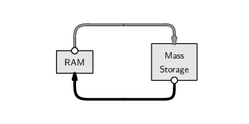
We will also look at some functions that go the other way and write a data structure from RAM to external mass storage.

9.7.1 The working directory

This section provides a little more information about how the R software environment works, with respect to reading and writing files.

Any files created during an R session are created in the current working directory of the session, unless an explicit path or folder or directory is specified. Similarly, when files are read into an R session, they are read from the current working directory.

On Linux, the working directory is the directory that the R session was started in. This means that the standard way to work on Linux is to create a directory for a particular project, put any relevant files in that directory, change into that directory, and then start an R session.

On Windows, it is typical to start R by double-clicking a shortcut or by selecting from the list of programs in the `Start' menu. This approach will, by default, set the working directory to one of the directories where R was installed, which is a bad place to work. Instead, it is a good idea to work in a separate directory for each project, create a shortcut to R within that directory, and set the `Start in' field on the properties dialog of the shortcut to be the directory for that project. An alternative is to use the setwd() function or the `Change dir' option on the `File' menu to explicitly change the working directory to something appropriate when working on a particular project.

9.7.2 Specifying files

In order to read or write a file, the first thing we need to be able to do is specify which file we want to work with. Any function that works with a file requires a precise description of the name of the file and the location of the file.

A filename is just a character value, e.g., "pointnemotemp.txt", but specifying the location of a file can involve a path, which describes a location on a persistent storage medium, such as a hard drive.

The best way to specify a path in R is via the file.path() function because this avoids the differences between path descriptions on different operating systems. For example, the following code generates a path to the file pointnemotemp.txt within the directory LAS (on a Linux system).

The file.choose() function can be used to allow interactive selection of a file. This is particularly effective on Windows because it provides a familiar file selection dialog box.

9.7.3 Text formats

R has functions for reading in the standard types of plain text formats: delimited formats, especially CSV files, and fixed-width formats (see Section 5.2). We will briefly describe the most important functions and then demonstrate their use in an example.

The read.table() function works for data in a delimited format. By default, the delimiter is whitespace (spaces and tabs), but an alternative may be specified via the sep argument. There is a read.csv() function for the special case of CSV files, and for data in a fixed-width format, there is the read.fwf() function.

The important arguments to these functions are the name of the external file and information about the format of the file. For example, in order to read a file in a fixed-width format with the read.fwf() function, we have to supply the widths of the fields in the file via the widths argument.

Another important piece of information required when reading text files is the data type of each column of data in the file. Everything in the file is text, including numeric values, which are stored as a series of digits, and this means that some of the text values from the file may need to be coerced so that they are stored as an appropriate data type in the resulting data frame.

The general rule is that, if all values within a column in the text file are numbers, then the values in that column are coerced to a numeric vector. Otherwise, the values are used to create a factor. Several arguments are provided to control the coercion from the text values in the file to a specific data type; we will see examples in the next section and in other case studies throughout this chapter.

Another function that can be used to read text files is the readLines() function. The result in this case is a character vector, where each line of the text file becomes a separate element of the vector. The text values from the file become text values within RAM, so no type coercion is necessary in this case.

This function is useful for processing a file that contains text, but not in a standard plain text format. For example, the readLines() function was used to read the HTML code from the World Population Clock web site in Section 9.1. Section 9.9 discusses tools for processing data that have been read into R as text.

The following case study provides some demonstrations of the use of these functions for reading text files.

9.7.4 Case study: Point Nemo (continued)

The temperature data obtained from NASA's Live Access Server for the Pacific Pole of Inaccessibility (see Section 1.1) were delivered in a plain text format (see Figure 9.5, which reproduces Figure 1.2 for convenience). How can we load this temperature information into R?

9.7.4.1 A read.table() example

One way to view the format of the file in Figure 9.5 is that the data start on the ninth line and data values within each row are separated by whitespace. This means that we can use the read.table() function to read the Point Nemo temperature information, as shown below.

In the above example, and in a number of examples throughout the rest of the chapter, the output displayed by R has been manually truncated to avoid wasting too much space on the page. This truncation is indicated by the use of ... at the end of a line of output, to indicate that there are further columns that are not shown, or ... on a line by itself, to indicate that there are further rows that are not shown.

**Figure 9.5:** The first few lines of the plain text output from the Live Access Server for the surface temperature at Point Nemo. This is a reproduction of Figure 1.2.
VARIABLE : Mean TS from clear sky composite (kelvin) FILENAME : ISCCPMonthly_avg.nc FILEPATH : /usr/local/fer_data/data/ SUBSET : 48 points (TIME) LONGITUDE: 123.8W(-123.8) LATITUDE : 48.8S 123.8W 23 16-JAN-1994 00 / 1: 278.9 16-FEB-1994 00 / 2: 280.0 16-MAR-1994 00 / 3: 278.9 16-APR-1994 00 / 4: 278.9 16-MAY-1994 00 / 5: 277.8 16-JUN-1994 00 / 6: 276.1 ...

Figure 9.5: The first few lines of the plain text output from the Live Access Server for the surface temperature at Point Nemo. This is a reproduction of Figure 1.2.

             VARIABLE : Mean TS from clear sky composite (kelvin)
             FILENAME : ISCCPMonthly_avg.nc
             FILEPATH : /usr/local/fer_data/data/
             SUBSET   : 48 points (TIME)
             LONGITUDE: 123.8W(-123.8)
             LATITUDE : 48.8S
                       123.8W 
                        23
 16-JAN-1994 00 /  1:  278.9
 16-FEB-1994 00 /  2:  280.0
 16-MAR-1994 00 /  3:  278.9
 16-APR-1994 00 /  4:  278.9
 16-MAY-1994 00 /  5:  277.8
 16-JUN-1994 00 /  6:  276.1
 ...

By default, read.table() assumes that the text file contains a data set with one case on each row and that each row contains multiple values, with each value separated by whitespace (one or more spaces or tabs). The skip argument is used to ignore the first few lines of a file when, for example, there is header information or metadata at the start of the file before the core data values.

The result of this function call is a data frame, with a variable for each column of values in the text file. In this case, there are four instances of whitespace on each line, so each line is split into five separate values, resulting in a data frame with five columns.

The types of variables are determined automatically. If a column only contains numbers, the variable is numeric; otherwise, the variable is a factor.

The names of the variables in the data frame can be read from the file, or specified explicitly in the call to read.table(). Otherwise, as in this case, R will generate a unique name for each column: V1, V2, V3, etc.

The result in this case is not perfect because we end up with several columns of junk that we do not want (V2 to V4). We can use a few more arguments to read.table() to improve things greatly.

> pointnemodelim <- 
       read.table(file.path("LAS", "pointnemotemp.txt"), 
                  skip=8, 
                  colClasses=c("character", 
                               "NULL", "NULL", "NULL", 
                               "numeric"),
                  col.names=c("date", "", "", "", "temp"))

The colClasses argument allows us to control the types of the variables explicitly. In this case, we have forced the first variable to be just text (these values are dates, not categories). There are five columns of values in the text file (treating whitespace as a column break), but we are not interested in the middle three, so we use "NULL" to indicate that these columns should just be ignored. The last column, the temperature values, is numeric.

It is common for the names of the variables to be included as the first line of a text file (the header argument can be used to read variable names from such a file). In this case, there is no line of column names in the file, so we provide the variable names explicitly, as a character vector, using the col.names argument.

The dates can be converted from character values to date values in a separate step using the as.Date() function.

The format argument contains special sequences that tell as.Date() where the various components of the date are within the character values. The %d means that there are two digits for the day, the %b means that the month is given as an abbreviated month name, and the %Y means that there are four digits for the year. The dashes are literal dash characters.

The way that these components map to the original character value for the first date is shown below.

Thus, for example, the original character value 16-JAN-1994 becomes the date value 1994-01-16.

9.7.4.2 A read.fwf() example

Another way to view the Point Nemo text file in Figure 9.5 is as a fixed-width format file. For example, the date values always reside in the first 12 characters of each line and the temperature values are always between character 24 and character 28. This means that we could also read the file using read.fwf(), as shown below.

> pointnemofwf <-
       read.fwf(file.path("LAS", "pointnemotemp.txt"), 
                skip=8,
                widths=c(-1, 11, -11, 5),
                colClasses=c("character", "numeric"),
                col.names=c("date", "temp"))

Again, the result is a data frame. As for the call to read.table(), we have specified the data type for each column, via the colClasses argument, and a name for each column, via col.names.

The widths argument specifies how wide each column of data is, with negative values used to ignore the specified number of characters. In this case, we have ignored the very first character on each line, we treat the next 11 characters as a date value, we ignore characters 13 to 23, and the final 5 characters are treated as the temp value.

The dates could be converted from character values to dates in exactly the same way as before.

9.7.4.3 A readLines() example

The two examples so far have demonstrated reading in the raw data for this data set, but so far we have completely ignored all of the metadata in the head of the file. This information is also very important and we would like to have some way to access it.

The readLines() function can help us here, at least in terms of getting raw text into R. The following code reads the first eight lines of the text file into a character vector.

Section 9.9 will describe some tools that could be used to extract the metadata values from this text.

9.7.4.4 A write.csv() example

As a simple demonstration of the use of functions that can write plain text files, we will now export the R data frame, pointnemodelim, to a new CSV file. This will create a much tidier plain text file that contains just the date and temperature values. Creating such a file is sometimes a necessary step in preparing a data set for analysis with a specific piece of analysis software.

The following code uses the write.csv() function to create a file called "pointnemoplain.csv" that contains the Point Nemo data (see Figure 9.6).

**Figure 9.6:** The first few lines of the plain text output from the Live Access Server for the surface temperature at Point Nemo in Comma-Separated Value (CSV) format. This is a reproduction of Figure 5.4.
date,temp 1994-01-16,278.9 1994-02-16,280 1994-03-16,278.9 1994-04-16,278.9 1994-05-16,277.8 1994-06-16,276.1 ...

The first argument in this function call is the data frame of values. The second argument is the name of the file to create.

The quote argument controls whether quote-marks are printed around character values and the row.names argument controls whether an extra column of unique names is printed at the start of each line. In both cases, we have turned these features off by specifying the value FALSE.

We will continue to use the Point Nemo data set, in various formats, throughout the rest of this section.

9.7.5 Binary formats

As discussed in Section 5.3, it is only possible to extract data from a binary file format with an appropriate piece of software that understands the particular binary format.

A number of R packages exist for reading particular binary formats. For example, the foreign package contains functions for reading files produced by other popular statistics software systems, such as SAS, SPSS, Systat, Minitab, and Stata. As an example of support for a more general binary format, the ncdf package provides functions for reading netCDF files.

We will look again at the Point Nemo temperature data (see Section 1.1), this time in a netCDF format, to demonstrate a simple use of the ncdf package.

The following code loads the ncdf package and reads the file pointnemotemp.nc.

One difference with this example compared to the functions in the previous section is that the result of reading the netCDF file is not a data frame.

This data structure is essentially a list that contains the information from the netCDF file. We can extract components of this list by hand, but a more convenient approach is to use several other functions provided by the ncdf package to extract the most important pieces of information from the ncdf data structure.

If we display the nemonc data structure, we can see that the file contains a single variable called Temperature.

> nemonc

file LAS/pointnemotemp.nc has 1 dimensions: 
Time   Size: 48 
------------------------ 
file LAS/pointnemotemp.nc has 1 variables: 
double Temperature[Time]  Longname:Temperature

> nemoTemps <- get.var.ncdf(nemonc, "Temperature")
> nemoTemps

 [1] 278.9 280.0 278.9 278.9 277.8 276.1 276.1 275.6 275.6
[10] 277.3 276.7 278.9 281.6 281.1 280.0 278.9 277.8 276.7
[19] 277.3 276.1 276.1 276.7 278.4 277.8 281.1 283.2 281.1
[28] 279.5 278.4 276.7 276.1 275.6 275.6 276.1 277.3 278.9
[37] 280.5 281.6 280.0 278.9 278.4 276.7 275.6 275.6 277.3
[46] 276.7 278.4 279.5

The netCDF file of Point Nemo data also contains information about the date that each temperature value corresponds to. This variable is called "Time". The following code reads this information from the file.

> nemoTimes <- get.var.ncdf(nemonc, "Time")
> nemoTimes

 [1]  8781  8812  8840  8871  8901  8932  8962  8993  9024
[10]  9054  9085  9115  9146  9177  9205  9236  9266  9297
[19]  9327  9358  9389  9419  9450  9480  9511  9542  9571
[28]  9602  9632  9663  9693  9724  9755  9785  9816  9846
[37]  9877  9908  9936  9967  9997 10028 10058 10089 10120
[46] 10150 10181 10211

This demonstrates that, even with binary file formats, it is often necessary to coerce data from the storage format that has been used in the file to a more convenient format for working with the data in RAM.

The netCDF format only allows numbers or text to be stored, so this date information has been stored in the file as numbers. However, additional information, metadata, can be stored along with the variable data in a netCDF file; netCDF calls this additional information “attributes”. In this case, the meaning of these numbers representing dates has been stored as the “units” attribute of this variable and the following code uses the att.get.ncdf() function to extract that attribute from the file.

> att.get.ncdf(nemonc, "Time", "units")

$hasatt
[1] TRUE

$value
[1] "number of days since 1970-01-01"

This tells us that the dates were stored as a number of days since January $1^{\rm st}$ 1970. Using this information, we can convert the numbers from the file back into real dates with the as.Date() function. The origin argument allows us to specify the meaning of the numbers.

In most cases, where a function exists to read a particular binary format, there will also be a function to write data out in that format. For example, the ncdf package also provides functions to save data from RAM to an external file in netCDF format.

9.7.6 Spreadsheets

When data is stored in a spreadsheet, one common approach is to save the data in a text format as an intermediate step and then read the text file into R using the functions from Section 9.7.3.

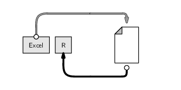
This makes the data easy to share, because text formats are very portable, but it has the disadvantage that another copy of the data is created.

This is less efficient in terms of storage space and it creates issues if the original spreadsheet is updated.

If changes are made to the original spreadsheet, at best, there is extra work to be done to update the text file as well. At worst, the text file is forgotten and the update does not get propagated to other places.

There are several packages that provide ways to directly read data from a spreadsheet into R. One example is the (Windows only) xlsReadWrite package, which includes the read.xls() function for reading data from an Excel spreadsheet.

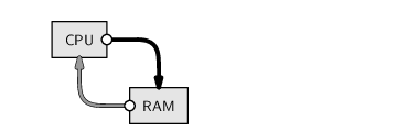
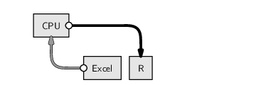
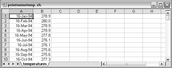
Figure 9.7 shows a screen shot of the Point Nemo temperature data (see Section 1.1) stored in a Microsoft Excel spreadsheet.

Notice that the date information has come across as numbers. This is another example of the type coercion that can easily occur when transferring between different formats.

As before, we can easily convert the numbers to dates if we know the reference date for these numbers. Excel represents dates as the number of days since the $0^{\rm th}$ of January 1900, so we can recover the real dates with the following code.

We have to subtract 2 in this calculation because the Excel count starts from the $0^{\rm th}$ rather than the $1^{\rm st}$ of January and because Excel thinks that 1900 was a leap year (apparently to be compatible with the Lotus 123 spreadsheet software). Sometimes, computer technology is not straightforward.

The gdata package provides another way to access Excel spreadsheets with its own read.xls() function and it is also possible to access Excel spreadsheets via a technology called ODBC (see Section 9.7.8).

9.7.7 XML

In this section, we look at how to get information that has been stored in an XML document into R.

Although XML files are plain text files, functions like read.table() from Section 9.7.3 are of no use because they only work with data that are arranged in a plain text format, with the data laid out in rows and columns within the file.

It is possible to read an XML document into R as a character vector using a standard function like readLines(). However, extracting the information from the text is not trivial because it requires knowledge of XML.

Fortunately, there is an R package called XML that contains functions for reading and extracting data from XML files into R.

We will use the Point Nemo temperature data, in an XML format, to demonstrate some of the functions from the XML package. Figure 9.8 shows one possible XML format for the the Point Nemo temperature data.

**Figure 9.8:** The first few lines of the surface temperature at Point Nemo in an XML format. This is a reproduction of Figure 5.16.
<?xml version="1.0"?> <temperatures> <variable>Mean TS from clear sky composite (kelvin)</variable> <filename>ISCCPMonthly_avg.nc</filename> <filepath>/usr/local/fer_dsets/data/</filepath> <subset>93 points (TIME)</subset> <longitude>123.8W(-123.8)</longitude> <latitude>48.8S</latitude> <case date="16-JAN-1994" temperature="278.9" /> <case date="16-FEB-1994" temperature="280" /> <case date="16-MAR-1994" temperature="278.9" /> <case date="16-APR-1994" temperature="278.9" /> <case date="16-MAY-1994" temperature="277.8" /> <case date="16-JUN-1994" temperature="276.1" /> ... </temperatures>

Figure 9.8: The first few lines of the surface temperature at Point Nemo in an XML format. This is a reproduction of Figure 5.16.

<?xml version="1.0"?>
<temperatures>
    <variable>Mean TS from clear sky composite (kelvin)</variable>
    <filename>ISCCPMonthly_avg.nc</filename>
    <filepath>/usr/local/fer_dsets/data/</filepath>
    <subset>93 points (TIME)</subset>
    <longitude>123.8W(-123.8)</longitude>
    <latitude>48.8S</latitude>
    <case date="16-JAN-1994" temperature="278.9" />
    <case date="16-FEB-1994" temperature="280" />
    <case date="16-MAR-1994" temperature="278.9" />
    <case date="16-APR-1994" temperature="278.9" />
    <case date="16-MAY-1994" temperature="277.8" />
    <case date="16-JUN-1994" temperature="276.1" />

    ...

</temperatures>

There are several approaches to working with XML documents in R using the XML package, but in this section, we will only consider the approach that allows us to use XPath queries (see Section 7.3.1).

The first thing to do is to read the XML document into R using the function xmlTreeParse().

It is important to point out that the data structure that is created in RAM by this code, nemoDoc, is not a data frame.

> class(nemoDoc)

[1] "XMLInternalDocument" "XMLAbstractDocument"
[3] "oldClass"

We must use other special functions from the XML package to work with this data structure.

In particular, the getNodeSet() function allows us to select elements from this data structure using XPath expressions.

In the following example, we extract the temperature attribute values from all case elements in the XML document. The XPath expression "/temperatures/case/@temperature" selects all of the temperature attributes of the case elements within the root temperatures element.

> nemoDocTempText <- 
       unlist(getNodeSet(nemoDoc, 
                         "/temperatures/case/@temperature"),
              use.names=FALSE)

The first argument to getNodeSet() is the data structure previously created by xmlParse() and the second argument is the XPath expression. The result of the call to getNodeSet() is a list and the call to unlist() converts the list to a vector.

One important point about the above result, nemoDocTempText, is that it is a character vector. This reflects the fact that everything is stored as text within an XML document. If we want to have numeric values to work with, we need to coerce these text values into numbers.

Before we do that, the following code shows how to extract the date values from the XML document as well. The only difference from the previous call is the XPath that we use.

> nemoDocDateText <- 
       unlist(getNodeSet(nemoDoc, 
                         "/temperatures/case/@date"), 
              use.names=FALSE)

Again, the values are all text, so we need to coerce them to dates. The following code performs the appropriate type coercions and combines the dates and temperatures into a data frame.

> data.frame(date=as.Date(nemoDocDateText, "%d-%b-%Y"),
              temp=as.numeric(nemoDocTempText))

With this approach to reading XML files, there is one final step: we need to signal that we are finished with the file by calling the free() function.

9.7.8 Databases

Very large data sets are often stored in relational databases. As with spreadsheets, a simple approach to extracting information from the database is to export it from the database to text files and work with the text files. This is an even worse option for databases than it was for spreadsheets because it is more common to extract just part of a database, rather than an entire spreadsheet. This can lead to several different text files from a single database, and these are even harder to maintain if the database changes.

A superior option is to extract information directly from the database management system into R.

There are packages for connecting directly to several major database management systems. Two main approaches exist, one based on the DBI package and one based on the RODBC package.

The DBI package defines a set of standard (generic) functions for communicating with a database, and a number of other packages, e.g., RMySQL and RSQLite, build on that to provide functions specific to a particular database system. The important functions to know about with this approach are:

The RODBC package defines functions for communicating with any ODBC (Open Database Connectivity) compliant software. This allows connections with many different types of software, including, but not limited to, most database management systems. For example, this approach can also be used to extract information from a Microsoft Excel spreadsheet.

The RODBC approach makes it possible to connect to a wider range of other software systems, but it may involve installation of additional software.

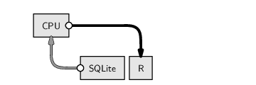
The simplest approach of all is provided by the RSQLite package because it includes the complete SQLite application, so no other software needs to be installed. However, this will only be helpful if the data are stored in an SQLite database.

9.7.9 Case study: The Data Expo (continued)

The Data Expo data set (see Section 5.2.8) contains several different atmospheric measurements, all measured at 72 different time periods and 576 different locations. These data have been stored in an SQLite database, with a table for location information, a table for time period information, and a table of the atmospheric measurements (see Section 7.1).

The following SQL code extracts information for the first two locations in the location table.

The following code carries out this query from within R. The first step is to connect to the database.

> result <- 
       dbGetQuery(con,
                  "SELECT *
                       FROM location_table
                       WHERE ID = 1 OR ID = 2")
> result

  ID longitude latitude elevation
1  1   -113.75    36.25   1526.25
2  2   -111.25    36.25   1759.56

Notice that the result is a data frame. The final step is to release our connection to SQLite.

Recap

For many binary formats and spreadsheets, there exist packages with special functions for reading files in the relevant format.

Several packages provide special functions for extracting data from relational databases. The result of a query to a database is a data frame.

two-digit day, `%d`:	`16-JAN-1994`
abbreviated month name, `%b`:	`16- JAN-1994`
four-digit year, `%Y`:	`16-JAN- 1994`
literal dashes:	`16 -JAN -1994`

9.7 Data import/export

9.7.1 The working directory

9.7.2 Specifying files

9.7.3 Text formats

9.7.4 Case study: Point Nemo (continued)

9.7.4.1 A `read.table()` example

9.7.4.2 A `read.fwf()` example

9.7.4.3 A `readLines()` example

9.7.4.4 A `write.csv()` example

9.7.5 Binary formats

9.7.6 Spreadsheets

9.7.7 XML

9.7.8 Databases

9.7.9 Case study: The Data Expo (continued)

Recap

9.7 Data import/export

9.7.1 The working directory

9.7.2 Specifying files

9.7.3 Text formats

9.7.4 Case study: Point Nemo (continued)

9.7.4.1 A read.table() example

9.7.4.2 A read.fwf() example

9.7.4.3 A readLines() example

9.7.4.4 A write.csv() example

9.7.5 Binary formats

9.7.6 Spreadsheets

9.7.7 XML

9.7.8 Databases

9.7.9 Case study: The Data Expo (continued)

Recap

9.7.4.1 A `read.table()` example

9.7.4.2 A `read.fwf()` example

9.7.4.3 A `readLines()` example

9.7.4.4 A `write.csv()` example