The previous section dealt with techniques that are useful for for manipulating a variety of data structures and a variety of data types.
This section is focused solely on data manipulation techniques for working with vectors containing character values.
Plain text is a very common format for storing information, so it is very useful to be able to manipulate text. It may be necessary to convert a data set from one text format to another. It is also common to search for and extract important keywords or specific patterns of characters from within a large set of text.
We will introduce some of the basic text processing ideas via a simple example.
One of the longest placenames in the world is attributed to a hill in the Hawke's Bay region of New Zealand. The name (in Maori) is ...
Taumatawhakatangihangakoauauotamateaturipukakapikimaungahoronukupokaiwhenuakitanatahu
... which means “The hilltop where Tamatea with big knees, conqueror of mountains, eater of land, traveler over land and sea, played his koauau [flute] to his beloved.”
Children at an Auckland primary school were given a homework assignment that included counting the number of letters in this name. This task of counting the number of characters in a piece of text is a simple example of what we will call text processing and is the sort of task that often comes up when working with data that have been stored in a text format.
Counting the number of characters in a piece of text is something that any programming language will do. Assuming that the name has been saved into a text file called placename.txt, here is how to use the scan() function to read the name into R, as a character vector of length 1.
> placename <- scan(file.path("Placename", "placename.txt"),
                     "character")
|
The first argument provides the name and location of the file and the second argument specifies what sort of data type is in the file. In this case, we are reading a single character value from a file.
We can now use the nchar() function to count the number of characters in this text.
> nchar(placename)
[1] 85
|
Counting characters is a very simple text processing task, though even with something that simple, performing the task using a computer is much more likely to get the right answer. We will now look at some more complex text processing tasks.
The homework assignment went on to say that, in Maori, the combinations `ng' and `wh' can be treated as a single letter. Given this, how many letters are in the placename? There are two possible approaches: convert every `ng' and `wh' to a single letter and recount the number of letters, or count the number of `ng's and `wh's and subtract that from the total number of characters. We will consider both approaches because they illustrate two different text processing tasks.
For the first approach, we could try counting all of the `ng's and `wh's as single letters by searching through the text and converting all of them into single characters and then redoing the count. In R, we can perform this search-and-replace task using the gsub() function, which takes three arguments: a pattern to search for, a replacement value, and the text to search within. The result is the original text with the pattern replaced. Because we are only counting letters, it does not matter which letter we choose as a replacement. First, we replace occurrences of `ng' with an underscore character.
> replacengs <- gsub("ng", "_", placename)
> replacengs
|
[1] "Taumatawhakata_iha_akoauauotamateaturipukakapikimau_ahoronukupokaiwhenuakitanatahu"
Next, we replace the occurrences of `wh' with an underscore character.
> replacewhs <- gsub("wh", "_", replacengs)
> replacewhs
|
[1] "Taumata_akata_iha_akoauauotamateaturipukakapikimau_ahoronukupokai_enuakitanatahu"
Finally, we count the number of letters in the resulting text.
> nchar(replacewhs)
[1] 80
|
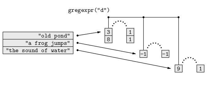
The alternative approach involves just finding out how many `ng's and `wh's are in the text and subtracting that number from the original count. This simple step of searching within text for a pattern is yet another common text processing task. There are several R functions that perform variations on this task, but for this example we need the function gregexpr() because it returns all of the matches within a piece of text. This function takes two arguments: a pattern to search for and the text to search within. The result is a vector of the starting positions of the pattern within the text, with an attribute that gives the lengths of each match. Figure 9.14 includes a diagram that illustrates how this function works.
> ngmatches <- gregexpr("ng", placename)[[1]]
> ngmatches
[1] 15 20 54
attr(,"match.length")
[1] 2 2 2
attr(,"useBytes")
[1] TRUE
|
This result shows that the pattern `ng' occurs three times in the placename, starting at character positions 15, 20, and 54, respectively, and that the length of the match is 2 characters in each case. Here is the result of searching for occurrences of `wh':
> whmatches <- gregexpr("wh", placename)[[1]]
> whmatches
[1]  8 70
attr(,"match.length")
[1] 2 2
attr(,"useBytes")
[1] TRUE
|
The return value of gregexpr() is a list to allow for more than one piece of text to be searched at once. In this case, we are only searching a single piece of text, so we just need the first component of the result.
We can use the length() function to count how many matches there were in the text.
> length(ngmatches)
[1] 3
|
> length(whmatches)
[1] 2
|
The final answer is simple arithmetic.
> nchar(placename) -
     (length(ngmatches) + length(whmatches))
[1] 80
|
For the final question in the homework assignment, the students had to count how many times each letter appeared in the placename (treating `wh' and `ng' as separate letters again).
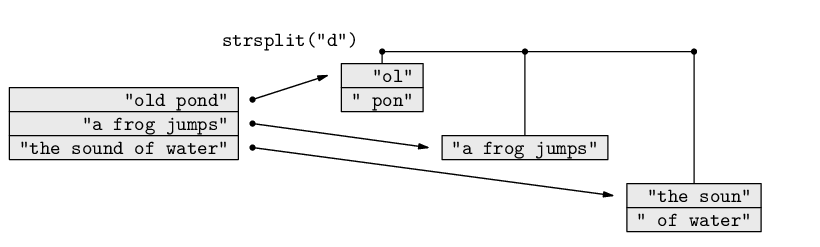
One way to do this in R is by breaking the placename into individual characters and creating a table of counts. Once again, we have a standard text processing task: breaking a single piece of text into multiple pieces. The strsplit() function performs this task in R. It takes two arguments: the text to break up and a pattern which is used to decide where to split the text. If we give the value NULL as the second argument, the text is split at each character. Figure 9.14 includes a diagram that illustrates how this function works.
> nameLetters <- strsplit(placename, NULL)[[1]]
> nameLetters
 [1] "T" "a" "u" "m" "a" "t" "a" "w" "h" "a" "k" "a" "t" "a"
[15] "n" "g" "i" "h" "a" "n" "g" "a" "k" "o" "a" "u" "a" "u"
[29] "o" "t" "a" "m" "a" "t" "e" "a" "t" "u" "r" "i" "p" "u"
[43] "k" "a" "k" "a" "p" "i" "k" "i" "m" "a" "u" "n" "g" "a"
[57] "h" "o" "r" "o" "n" "u" "k" "u" "p" "o" "k" "a" "i" "w"
[71] "h" "e" "n" "u" "a" "k" "i" "t" "a" "n" "a" "t" "a" "h"
[85] "u"
|
Again, the result is a list to allow for breaking up multiple pieces of text at once. In this case, because we only have one piece of text, we are only interested in the first component of the list.
One minor complication is that we want the uppercase `T' to be counted as a lowercase `t'. The function tolower() performs this task.
> lowerNameLetters <- tolower(nameLetters)
> lowerNameLetters
 [1] "t" "a" "u" "m" "a" "t" "a" "w" "h" "a" "k" "a" "t" "a"
[15] "n" "g" "i" "h" "a" "n" "g" "a" "k" "o" "a" "u" "a" "u"
[29] "o" "t" "a" "m" "a" "t" "e" "a" "t" "u" "r" "i" "p" "u"
[43] "k" "a" "k" "a" "p" "i" "k" "i" "m" "a" "u" "n" "g" "a"
[57] "h" "o" "r" "o" "n" "u" "k" "u" "p" "o" "k" "a" "i" "w"
[71] "h" "e" "n" "u" "a" "k" "i" "t" "a" "n" "a" "t" "a" "h"
[85] "u"
|
Now it is a simple matter of calling the tablefunction to produce a table of counts of the letters.
> letterCounts <- table(lowerNameLetters)
> letterCounts
lowerNameLetters
 a  e  g  h  i  k  m  n  o  p  r  t  u  w
22  2  3  5  6  8  3  6  5  3  2  8 10  2
|
As well as pulling text apart into smaller pieces as we have done so far, we also need to be able to put several pieces of text together to make a single larger piece of text.
For example, if we begin with the individual letters of the placename, as in the character vector nameLetters, how do we combine the letters to make a single character value? In R, this can done with the paste() function.
The paste() function can be used to combine separate character vectors or to combine the character values within a single character vector. In this case, we want to perform the latter task.
We have a character vector containing 85 separate character values.
> nameLetters
 [1] "T" "a" "u" "m" "a" "t" "a" "w" "h" "a" "k" "a" "t" "a"
[15] "n" "g" "i" "h" "a" "n" "g" "a" "k" "o" "a" "u" "a" "u"
[29] "o" "t" "a" "m" "a" "t" "e" "a" "t" "u" "r" "i" "p" "u"
[43] "k" "a" "k" "a" "p" "i" "k" "i" "m" "a" "u" "n" "g" "a"
[57] "h" "o" "r" "o" "n" "u" "k" "u" "p" "o" "k" "a" "i" "w"
[71] "h" "e" "n" "u" "a" "k" "i" "t" "a" "n" "a" "t" "a" "h"
[85] "u"
|
The following code combines the individual character values to make the complete placename. The collapse argument specifies that the character vector should be collapsed into a single character value with, in this case (collapse=""), nothing in between each character.
> paste(nameLetters, collapse="")
|
[1] "Taumatawhakatangihangakoauauotamateaturipukakapikimaungahoronukupokaiwhenuakitanatahu"
This section has introduced a number of functions for counting letters in text, transforming text, breaking text apart, and putting it back together again. More examples of the use of these functions are given in the next section and in case studies later on.
Two of the tasks we looked at when working with the long Maori placename in the previous case study involved treating both `ng' and `wh' as if they were single letters by replacing them both with underscores. We performed the task in two steps: convert all occurrences of `ng' to an underscore, and then convert all occurrences of `wh' to an underscore. Conceptually, it would be simpler, and more efficient, to perform the task in a single step: convert all occurrences of `ng' and `wh' to underscore characters. Regular expressions allow us to do this.
With the placename in the variable called placename, converting both `ng' and `wh' to underscores in a single step is achieved as follows:
> gsub("ng|wh", "_", placename)
|
[1] "Taumata_akata_iha_akoauauotamateaturipukakapikimau_ahoronukupokai_enuakitanatahu"
The regular expression we are using, ng|wh, describes a pattern: the character `n' followed by the character `g' or the character `w' followed by the character `h'. The vertical bar, |, is a metacharacter. It does not have its normal meaning, but instead denotes an optional pattern; a match will occur if the text contains either the pattern to the left of the vertical bar or the pattern to the right of the vertical bar. The characters `n', `g', `w', and `h' are all literals; they have their normal meaning.
A regular expression consists of a mixture of literal characters, which have their normal meaning, and metacharacters, which have a special meaning. The combination describes a pattern that can be used to find matches amongst text values.
A regular expression may be as simple as a literal word, such as cat, but regular expressions can also be quite complex and express sophisticated ideas, such as [a-z]{3,4}[0-9]{3}, which describes a pattern consisting of either three or four lowercase letters followed by any three digits.
Just like all of the other technologies in this book, there are several different versions of regular expressions, however, rather than being numbered, the different versions of regular expressions have different names: there are Basic regular expressions, Extended (POSIX) regular expressions, and Perl-Compatible regular expressions (PCRE). We will assume Extended regular expressions in this book, though for the level of detail that we encounter, the differences between Extended regular expressions and PCRE are not very important. Basic regular expressions, as the name suggests, have fewer features than the other versions.
There are two important components required to use regular expressions: we need to be able to write regular expressions and we need software that understands regular expressions in order to search text for the pattern specified by the regular expression.
We will focus on the use of regular expressions with R in this book, but there are many other software packages that understand regular expressions, so it should be possible to use the information in this chapter to write effective regular expressions within other software environments as well. One caveat is that R consumes backslashes in text, so it is necessary to type a double backslash in order to obtain a single backslash in a regular expression. This means that we often avoid the use of backslashes in regular expressions in R and, when we are forced to use backslashes, the regular expressions will look more complicated than they would in another software setting.
Something to keep in mind when writing regular expressions (especially when trying to determine why a regular expression is not working) is that most software that understands regular expressions will perform “eager” and “greedy” searches. This means that the searches begin from the start of a piece of text, the first possible match succeeds (even if a “better” match might exist later in the text), and as many characters as possible are matched. In other words, the first and longest possible match is found by each component of a regular expression. A common problem is to have a later component of a regular expression fail to match because an earlier component of the expression has consumed the entire piece of text all by itself.
For this reason, it is important to remember that regular expressions are a small computer language of their own and should be developed with just as much discipline and care as we apply to writing any computer code. In particular, a complex regular expression should be built up in smaller pieces in order to understand how each component of the regular expression works before adding further components.
The next case study looks at some more complex uses and provides some more examples. Chapter 11 describes several other important metacharacters that can be used to build more complex regular expressions.
As part of a series of field trials conducted by the Institut du Végétal in France,9.3data were gathered on the effect of the disease Septoria tritici on wheat. The amount of disease on individual plants was recorded using data collection forms that were filled in by hand by researchers in the field.
In 2007, due to unusual climatic conditions, two other diseases, Puccinia recondita (“brown rust”) and Puccinia striiformis (“yellow rust”) were also observed to be quite prevalent. The data collection forms had no specific field for recording the amount of rust on each wheat plant, so data were recorded ad hoc in a general area for “diverse observations”.
In this case study, we will not be interested in the data on Septoria tritici. Those data were entered into a standard form using established protocols, so the data were relatively tidy.
Instead, we will focus on the yellow rust and brown rust data because these data were not anticipated, so the data were recorded quite messily. The data included other comments unrelated to rust and there were variations in how the rust data were expressed by different researchers.
This lack of structure means that the rust data cannot be read into R using the functions that expect a regular format, such as read.table() and read.fwf() (see Section 9.7.3). This provides us with an example where text processing tools allow us to work with data that have an irregular structure.
The yellow and brown rust data were transcribed verbatim into a plain text file, as shown in Figure 9.15.
Fortunately, for the purposes of recovering these results, some basic features of the data are consistent.
Each line of data represents one wheat plant. If brown rust was present, the line contains the letters rb, followed by a space, followed by a number indicating the percentage of the plant affected by the rust (possibly with a percentage sign). If the plant was afflicted by yellow rust, the same pattern applies except that the letters rj are used. It is possible for both diseases to be present on the same plant (see the last line of data in Figure 9.15).
|
lema, rb 2%
rb 2%
rb 3%
rb 4%
rb 3%
rb 2%,mineuse
rb
rb
rb 12
rb
rj 30%
rb
rb
rb 25%
rb
rb
rb
rj 10, rb 4
|
The abbreviations rb and rj were used because the French common names for the diseases are rouille brune and rouille jaune.
For this small set of recordings, the data could be extracted by hand. However, the full data set contains many more records so we will develop a code solution that uses regular expressions to recover the rust data from these recordings.
The first step is to get the data into R. We can do this using the readLines() function, which will create a character vector with one element for each line of recordings.
> wheat <- readLines(file.path("Wheat", "wheat.txt"))
> wheat
 [1] "lema, rb 2%"   "rb 2%"         "rb 3%"
 [4] "rb 4%"         "rb 3%"         "rb 2%,mineuse"
 [7] "rb"            "rb"            "rb 12"
[10] "rb"            "rj 30%"        "rb"
[13] "rb"            "rb 25%"        "rb"
[16] "rb"            "rb"            "rj 10, rb 4"
|
What we want to end up with are two variables, one recording the amount of brown rust on each plant and one recording the amount of yellow rust.
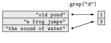
Starting with brown rust, the first thing we could do is find out which plants have any brown rust on them. The following code does this using the grep() function. The result is a vector of indices that tells us which lines contain the pattern we are searching for. Figure 9.14 includes a diagram that illustrates how this function works.
> rbLines <- grep("rb [0-9]+", wheat)
> rbLines
[1] 1 2 3 4 5 6 9 14 18
|
The regular expression in this call demonstrates two more important examples of metacharacters. The square brackets, `[' and `]', are used to describe a character set that will be matched. Within the brackets we can specify individual characters or, as in this case, ranges of characters; 0-9 means any character between `0' and `9'.
The plus sign, `+', is also a metacharacter, known as a modifier. It says that whatever immediately precedes the plus sign in the regular expression can repeat several times. In this case, [0-9]+ will match one or more digits.
The letters `r', `b', and the space are all literal, so the entire regular expression will match the letters rb, followed by a space, followed by one or more digits. Importantly, this pattern will match anywhere within a line; the line does not have to begin with rb. In other words, this will match rows on which brown rust has been observed on the wheat plant.
Having found which lines contain information about brown rust, we want to extract the information from those lines. The indices from the call to grep() can be used to subset out just the relevant lines of data.
> wheat[rbLines]
[1] "lema, rb 2%"   "rb 2%"         "rb 3%"
[4] "rb 4%"         "rb 3%"         "rb 2%,mineuse"
[7] "rb 12"         "rb 25%"        "rj 10, rb 4"
|
We will extract just the brown rust information from these lines in two steps, partly so that we can explore more about regular expressions, and partly because we have to in order to cater for plants that have been afflicted by both brown and yellow rust.
The first step is to reduce the line down to just the information about brown rust. In other words, we want to discard everything except the pattern that we are looking for, rb followed by a space, followed by one or more digits. The following code performs this step.
> rbOnly <- gsub("^.*(rb [0-9]+).*$", "\\1",
                  wheat[rbLines])
> rbOnly
[1] "rb 2"  "rb 2"  "rb 3"  "rb 4"  "rb 3"  "rb 2"  "rb 12"
[8] "rb 25" "rb 4"
|
The overall strategy being used here is to match the entire line of text, from the first character to the last, but within that line we want to identify and isolate the important component of the line, the brown rust part, so that we can retain just that part.
Again, we have some new metacharacters to explain. First is the “hat” character, `^', which matches the start of the line (or the start of the text). Next is the full stop, `.'. This will match any single character, no matter what it is. The `*' character is similar to the `+'; it modifies the immediately preceding part of the expression and allows for zero or more occurrences. An expression like ^.* allows for any number of characters at the start of the text (including zero characters, or an empty piece of text).
The parentheses, `(' and `)', are used to create subpatterns within a regular expression. In this case, we are isolating the pattern rb [0-9]+, which matches the brown rust information that we are looking for. Parentheses are useful if we want a modifier, like `+' or `*', to affect a whole subpattern rather than a single character, and they can be useful when specifying the replacement text in a search-and-replace operation, as we will see below.
After the parenthesized subpattern, we have another .* expression to allow for any number of additional characters and then, finally, a dollar sign, `$'. The latter is the counterpart to `^'; it matches the end of a piece of text.
Thus, the complete regular expression explicitly matches an entire piece of text that contains information on brown rust. Why do we want to do this? Because we are going to replace the entire text with only the piece that we want to keep. That is the purpose of the backreference, "\\1", in the replacement text.
The text used to replace a matched pattern in gsub() is mostly just literal text. The one exception is that we can refer to subpatterns within the regular expression that was used to find a match. By specifying "\\1", we are saying reuse whatever matched the subpattern within the first set of parentheses in the regular expression. This is known as a backreference. In this case, this refers to the brown rust information.
The overall meaning of the gsub() call is therefore to replace the entire text with just the part of the text that contains the information about brown rust.
Now that we have character values that contain only the brown rust information, the final step we have to perform is to extract just the numeric data from the brown rust information. We will do this in three ways in order to demonstrate several different techniques.
One approach is to take the text values that contain just the brown rust information and throw away everything except the numbers. The following code does this using a regular expression.
> gsub("[^0-9]", "", rbOnly)
[1] "2" "2" "3" "4" "3" "2" "12" "25" "4"
|
The point about this regular expression is that it uses ^ as the first character within the square brackets. This has the effect of negating the set of characters within the brackets, so [^0-9] means any character that is not a digit. The effect of the complete gsub() call is to replace anything that is not a digit with an empty piece of text, so only the digits remain.
An alternative approach is to recognize that the text values that we are dealing with have a very regular structure. In fact, all we need to do is drop the first three characters from each piece of text. The following code does this with a simple call to substring().
> substring(rbOnly, 4)
[1] "2" "2" "3" "4" "3" "2" "12" "25" "4"
|
The first argument to substring() is the text to reduce and the second argument specifies which character to start from. In this case, the first character we want is character 4. There is an optional third argument that specifies which character to stop at, but if, as in this example, the third argument is not specified, then we keep going to the end of the text.
The name of this function comes from the fact that text values, or character values, are also referred to as strings.
The final approach that we will consider works with the entire original text, wheat[rbLines], and uses a regular expression containing an extra set of parentheses to isolate just the numeric content of the brown rust information as a subpattern of its own. The replacement text refers to this second subpattern, "\\2", so it reduces the entire line to only the part of the line that is the numbers within the brown rust information, in a single step.
> gsub("^.*(rb ([0-9]+)).*$", "\\2", wheat[rbLines])
[1] "2" "2" "3" "4" "3" "2" "12" "25" "4"
|
We are not quite finished because we want to produce a variable that contains the brown rust information for all plants. We will use NA for plants that were not afflicted.
A simple way to do this is to create a vector of NAs and then fill in the rows for which we have brown rust information. The other important detail in the following code is the conversion of the textual information into numeric values using as.numeric().
> rb <- rep(NA, length(wheat))
> rb[rbLines] <- as.numeric(gsub("^.*(rb ([0-9]+)).*$",
                                  "\\2", wheat[rbLines]))
> rb
[1] 2 2 3 4 3 2 NA NA 12 NA NA NA NA 25 NA NA NA 4
|
To complete the exercise, we need to repeat the process for yellow rust. Rather than repeat the approach used for brown rust, we will investigate a different solution, which will again allow us to demonstrate more text processing techniques.
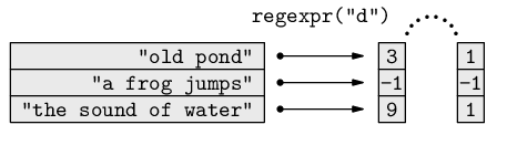
This time, we will use regexpr() rather than grep() to find the lines that we want. We are now searching for the lines containing yellow rust data.
> rjData <- regexpr("rj [0-9]+", wheat)
> rjData
 [1] -1 -1 -1 -1 -1 -1 -1 -1 -1 -1  1 -1 -1 -1 -1 -1 -1  1
attr(,"match.length")
 [1] -1 -1 -1 -1 -1 -1 -1 -1 -1 -1  5 -1 -1 -1 -1 -1 -1  5
attr(,"useBytes")
[1] TRUE
|
The result is a numeric vector with a positive number for lines that contain yellow rust data and -1 otherwise. The number indicates the character where the data start. Figure 9.14 includes a diagram that illustrates how this function works.
In this case, there are only two lines containing yellow rust data (lines 11 and 18) and, in both cases, the data start at the first character.
The result also has an attribute called match.length, which contains the number of characters that produced the match with the regular expression that we were searching for. In both cases, the pattern matched a total of 5 characters: the letters r and j, followed by a space, followed by two digits. This length information is particularly useful because it will allow us to extract the yellow rust data immediately using substring(). This time we specify both a start and an end character for the subset of the text.
> rjText <- substring(wheat, rjData,
                       attr(rjData, "match.length"))
> rjText
 [1] ""      ""      ""      ""      ""      ""      ""
 [8] ""      ""      ""      "rj 30" ""      ""      ""
[15] ""      ""      ""      "rj 10"
|
Obtaining the actual numeric data can be carried out using any of the techniques we described above for the brown rust case.
The following code produces the final result, including both brown and yellow rust as a data frame.
> rj <- as.numeric(substring(rjText, 4))
> data.frame(rb=rb, rj=rj)
   rb rj
1   2 NA
2   2 NA
3   3 NA
4   4 NA
5   3 NA
6   2 NA
7  NA NA
8  NA NA
9  12 NA
10 NA NA
11 NA 30
12 NA NA
13 NA NA
14 25 NA
15 NA NA
16 NA NA
17 NA NA
18  4 10
|
Paul Murrell

This work is licensed under a Creative Commons Attribution-Noncommercial-Share Alike 3.0 New Zealand License.