As we have seen in most of the sections so far in this chapter, most of the tasks that we perform with data, using a programming language, work with the data in RAM. We access data structures that have been stored in RAM and we create new data structures in RAM.
Something that we have largely ignored to this point is how we get to see the data on the computer screen.
The purpose of this section is to address the topic of formatting data values for display.
The important thing to keep in mind is that we do not typically see raw computer memory on screen; what we see is a display of the data in a format that is fit for human consumption.
There are two main ways that information is displayed on a computer screen: as text output or as graphical output (pictures or images). R has sophisticated facilities for graphical output, but that is beyond the scope of this book and we will not discuss those facilities here. Instead, we will focus on displaying text output to the screen.
For a start, we will look a little more closely at how R automatically displays values on the screen.
In this section we will work with a subset of the temperature values from the Point Nemo data set (see Section 1.1).
The temperature values have previously been read into R as the temp variable in the data frame called pointnemodelim (see Section 9.7.4). In this section, we will only work with the first 12 of these temperature values, which represent the first year's worth of monthly temperature recordings.
> twelveTemps <- pointnemodelim$temp[1:12]
> twelveTemps
 [1] 278.9 280.0 278.9 278.9 277.8 276.1 276.1 275.6 275.6
[10] 277.3 276.7 278.9
|
The data structure that we are dealing with is a numeric vector. The values in twelveTemps are stored in RAM as numbers.
However, the display that we see on screen is text. The values are numeric, so the characters in the text are mostly digits, but it is important to realize that everything that R displays on screen for us to read is a text version of the data values.
The function that displays text versions of data values on screen is called print(). This function gets called automatically to display the result of an R expression, but we can also call it directly, as shown below. The display is exactly the same as when we type the name of the symbol by itself.
> print(twelveTemps)
 [1] 278.9 280.0 278.9 278.9 277.8 276.1 276.1 275.6 275.6
[10] 277.3 276.7 278.9
|
One reason for calling print() directly is that this function has arguments that control how values are displayed on screen. For example, when displaying numeric values, there is an argument digits that controls how many significant digits are displayed.
In the following code, we use the digits argument to only display three digits for each temperature value. This has no effect on the values in RAM; it only affects how the numbers are converted to text for display on the screen.
> print(twelveTemps, digits=3)
[1] 279 280 279 279 278 276 276 276 276 277 277 279
|
The print() function is a generic function (see Section 9.6.8), so what gets displayed on screen is very different for different sorts of data structures; the arguments that provide control over the details of the display will also vary.
Although print() has some arguments that control how information is displayed, it is not completely flexible. For example, when printing out a numeric vector, as above, it will always print out the index, in this case [1], at the start of the line.
If we want to have complete control over what gets displayed on the screen, we need to perform the task in two steps: first, generate the text that we want to display, and then call the cat() function to display the text on the screen.
For simple cases, the cat() function will automatically coerce values to a character vector. For example, the following code uses cat() to display the twelveTemps numeric vector on screen. The fill argument says that a new line should be started after 60 characters have been used.
> cat(twelveTemps, fill=60)
278.9 280 278.9 278.9 277.8 276.1 276.1 275.6 275.6 277.3
276.7 278.9
|
The difference between this display and what print() displays is that there is no index at the start of each row. This is the usefulness of cat(): it just displays values and does not perform any formatting of its own. This means that we can control the formatting when we generate text values and then just use cat() to get the text values displayed on screen.
In summary, the problem of producing a particular display on screen is essentially a problem of generating a character vector in the format that we require and then calling cat().
The next section looks at the problem of generating character vectors in a particular format.
We have previously seen two ways to convert data values to character values: some functions, e.g., as.character(), perform an explicit type coercion from an original data structure to a character vector; and some functions, e.g., paste(), automatically coerce their arguments to character vectors. In this section, we will look at some more functions that perform explicit coercion to character values.
The following code coerces the twelveTemps numeric vector to a character vector using as.character().
> as.character(twelveTemps)
 [1] "278.9" "280"   "278.9" "278.9" "277.8" "276.1" "276.1"
 [8] "275.6" "275.6" "277.3" "276.7" "278.9"
|
One thing to notice about this result is that the second value, "280", is only three characters long, whereas all of the other values are five characters long.
This is a small example of a larger problem that arises when converting values, particularly numbers, to text; there are often many possible ways to perform the conversion. In the case of converting a real number to text, one major problem is how many decimal places to use.
There are several functions in R that we can use to resolve this problem.
The format() function produces character values that have a “common format.” What that means depends on what sorts of values are being formatted, but in the case of a numeric vector, it means that the resulting character values are all of the same length. In the following result, the second value is five characters long, just like all of the other values.
> format(twelveTemps)
 [1] "278.9" "280.0" "278.9" "278.9" "277.8" "276.1" "276.1"
 [8] "275.6" "275.6" "277.3" "276.7" "278.9"
|
The format() function has several arguments that provide some flexibility in the result, but its main benefit is that it displays all values with a common appearance.
For complete control over the conversion to text values, there is the sprintf() function.
The following code provides an example of the use of sprintf() that converts the twelveTemps numeric vector into a character vector where every numeric value is converted to a character value with two decimal places and a total of nine characters, followed by a space and a capital letter `K' (for degrees Kelvin).
> sprintf(fmt="%9.2f K", twelveTemps)
 [1] "   278.90 K" "   280.00 K" "   278.90 K" "   278.90 K"
 [5] "   277.80 K" "   276.10 K" "   276.10 K" "   275.60 K"
 [9] "   275.60 K" "   277.30 K" "   276.70 K" "   278.90 K"
|
The first argument to sprintf(), called fmt, defines the formatting of the values. The value of this argument can include special codes, like %9.2f. The first special code within the fmt argument is used to format the second argument to sprintf(), in this case the numeric vector twelveTemps.
There are a number of special codes for controlling the formatting of different types of values; the components of the format in this example are shown below.
| start of special code: | %9.2f K |
| real number format: | %9.2 f K |
| nine characters in total: | % 9.2f K |
| two decimal places: | %9 .2f K |
| literal text: | %9.2f K |
With the twelveTemps formatted like this, we can now use cat() to display the values on the screen in a format that is quite different from the display produced by print().
> twelveTemps
 [1] 278.9 280.0 278.9 278.9 277.8 276.1 276.1 275.6 275.6
[10] 277.3 276.7 278.9
|
> cat(sprintf("%9.2f K", twelveTemps), fill=60)
   278.90 K    280.00 K    278.90 K    278.90 K    277.80 K
   276.10 K    276.10 K    275.60 K    275.60 K    277.30 K
   276.70 K    278.90 K
|
This sort of formatting can also be useful if we need to generate a plain text file with a particular format. Having generated a character vector as above, this can easily be written to an external text file using the writeLines() function or by specifying a filename for cat() to write to. If the file argument is specified in a call to cat(), then output is written to an external file rather than being displayed on the screen.
One reason for using a particular format for displaying results is so that the results can be conveniently included in a research report.
For example, way back in Section 2.1, we saw a very basic web page report about the Pacific and Eurasian Poles of Inaccessibility. The web page is reproduced in Figure 9.16.
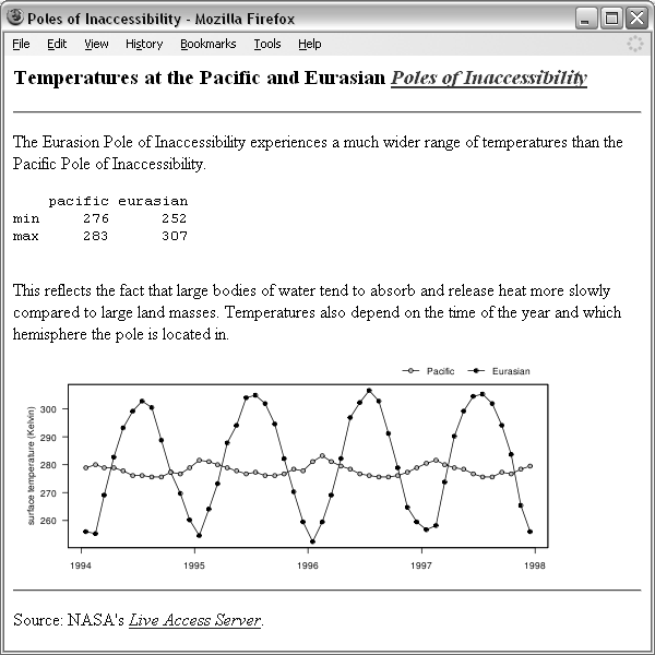 |
This web page includes a summary table showing the range of temperature values for both Poles of Inaccessibility. R code that generates the table of ranges is shown below.
> pointnemotemps <-
       read.fwf(file.path("LAS", "pointnemotemp.txt"),
                skip=8, widths=c(-23, 5),
                col.names=c("temp"))
> eurasiantemps <-
       read.fwf(file.path("LAS", "eurasiantemp.txt"),
                skip=8, widths=c(-23, 5),
                col.names=c("temp"))
> allTemps <- cbind(pacific=pointnemotemps$temp,
                     eurasian=eurasiantemps$temp)
> ranges <- round(rbind(min=apply(allTemps, 2, min),
                         max=apply(allTemps, 2, max)))
> ranges
    pacific eurasian
min     276      252
max     283      307
|
The HTML code that includes this table in the web page is reproduced below. This is the most basic way to make use of R output; simply copy the R display directly into another document, with a monospace font.
    <pre>
    pacific eurasian
min     276      252
max     283      307
    </pre>
However, this approach produces a very plain display. A more sophisticated approach is to format the R result using the same technology as is used to produce the report. For example, in the case of a web page report, we could create an HTML table to display the result.
Several R packages provide functions to carry out this task. For example, the hwriter package has an hwrite() function that converts an R table into text describing an HTML table.
> library(hwriter)
> cat(hwrite(ranges))
<table border="1">
<tr>
<td></td><td>pacific</td><td>eurasian</td></tr>
<tr>
<td>min</td><td>276</td><td>252</td></tr>
<tr>
<td>max</td><td>283</td><td>307</td></tr>
</table>
|
This approach allows us to integrate R results within a report more naturally and more aesthetically.
It is worth noting that this is just a text processing task; we are converting the values from the R table into text values and then combining those text values with HTML tags, which are just further text values.
This is another important advantage of carrying out tasks by writing computer code; we can use a programming language to write computer code. We can write code to generate our instructions to the computer, which is a tremendous advantage if the instructions are repetitive, for example, if we write the same HTML report every month.
Another option for producing HTML code from R data structures is the xtable package; this package can also format R data structures as LATEX tables.
Although a detailed description is beyond the scope of this book, it is also worth mentioning the Sweave package, which allows HTML (or LATEX) code to be combined with R code within a single document, thereby avoiding having to cut-and-paste results from R to a separate report document by hand.
The conversion of data values to a text representation is sometimes ambiguous and requires us to provide a specification of what the result should be.
It is possible to format the display of R data structures so that they can be integrated nicely within research reports.
Paul Murrell

This work is licensed under a Creative Commons Attribution-Noncommercial-Share Alike 3.0 New Zealand License.