New Results

45 Days data: 2¹⁸ data points

Non-MPI Results

Here are some trace and density plots I obtained for MLDC 1B.3.2. I used datasets of two different lengths that is 45 days long (2¹⁸ observations) and one year long datasets (2²¹). The plots are in two formats, pdf and png. Click on figure to view it in pdf. For each MCMC run the trace and density plots are just side by side. The densities are plotted in 5x3 pattern i.e. the first row has three densities for the first three chains and so on.

Figure 1. NON-MPI: MCMC Chain plot. For PDF format click on figure.

The above plot is for one non-mpi MCMC chain ran over a 45 days dataset (2^18 data points). The plot shows that for some of the parameters the chain is in stable status but sampling from wrong place.

I tried to know as to what happens to MCMC chains if we heatup the likelihood by taking some high index. The following graph again shows the trace plots of a non-mpi version MCMC but with heated likelihood. Here I ran two parallel chains with non-mpi (non-mpi: no massage passing inteface) but I used a temperature index of 1.9 so that to heatup the likelihood to melt down the density to some good extent. I got an impression that some parameters may converge to to the true value if we use higher temperatures. I this plot we can see that phiz (initial azimuthal orbital phase) is having quite big jumps but its not the case. Its actually because of angular range adjustment, that is when a particular angle gets out of its specified range (e.g. [0, pi] or [0, 2pi]) then its brought back by adding or subtarcting pi or 2pi. I don't think that its a reasonable strategy rather we can reject that proposed value for that particular angle leaving the proposed values in that same overall proposal intact since there is no harm to the properties MCMC (Renate in an oral discussion).

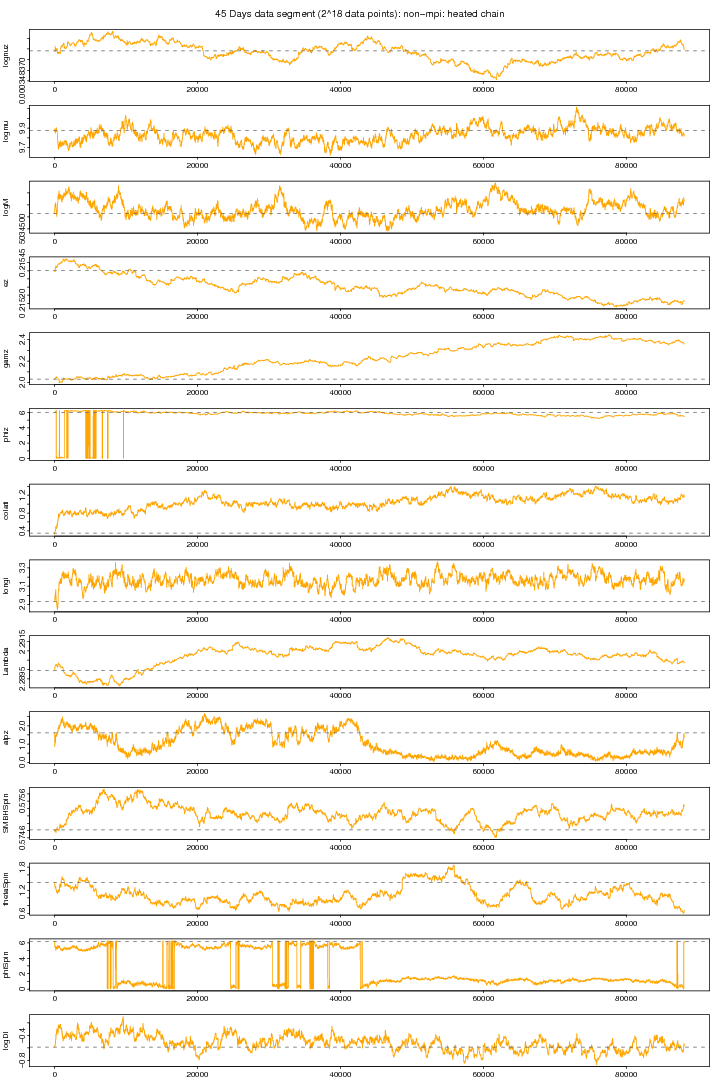
Figure 2. NON-MPI: Hot chain plot. For PDF format click on figure.

Combining the above two plots (see below) we can see that for some parameters the heated chain (orange) moves around the true values. Though the chains of some parameters are still distracted. (This problem seems to be solved in 10 MPI chains.)

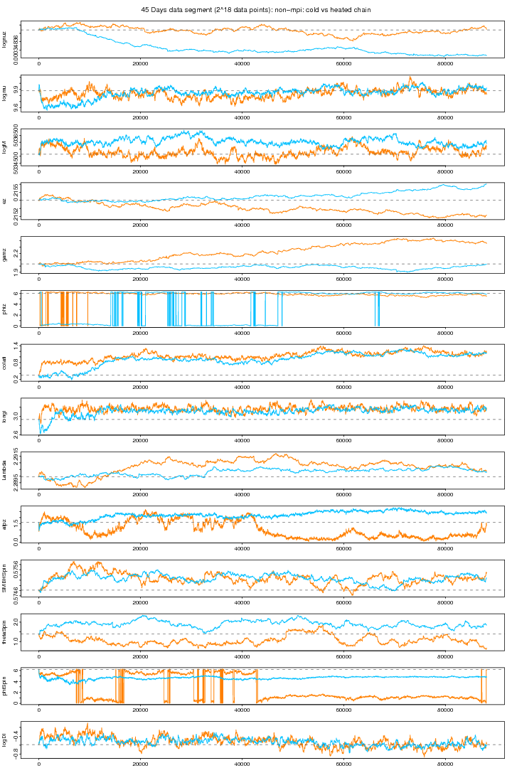
Figure 3. NON-MPI: Both cold and hot chains. For PDF format click on figure.

MPI Results

Following graph shows the trace plots of the first chain in a 10 chains MCMC run with MPI on the same data segment. These plots show that for some parameters such as phiz, latitude, longitude,Lambda, aplz, SMBHSpin and Distance the chain attains a very a good convergence. The other parameters also shows improved stabilitiy and mixing though its not visible because its very small sample comapared to the size of the jumps proposed (small jumps need a longer MCMC run). From extensive trial and error study I found a proposal covariance matrix which I think is very good than before. The ordinary Identity Unit matrix does not work at all here. You need to be sure that for a particular vector of proposed values an EMRI is generated. The parameters whose slightest dis-agreement can leed to no-EMRI-generation (or even if generated, takes a long time thus increasing the time per iteration) are nu (orbital frequency), ez (eccentricity), SMBH Spin and thetaSpin (polar angle of spin). While a big jump in Lambda (Direction of the Orbital Angular Momentum) brings a tremondous reduction in MCMC proposal acceptance rate.

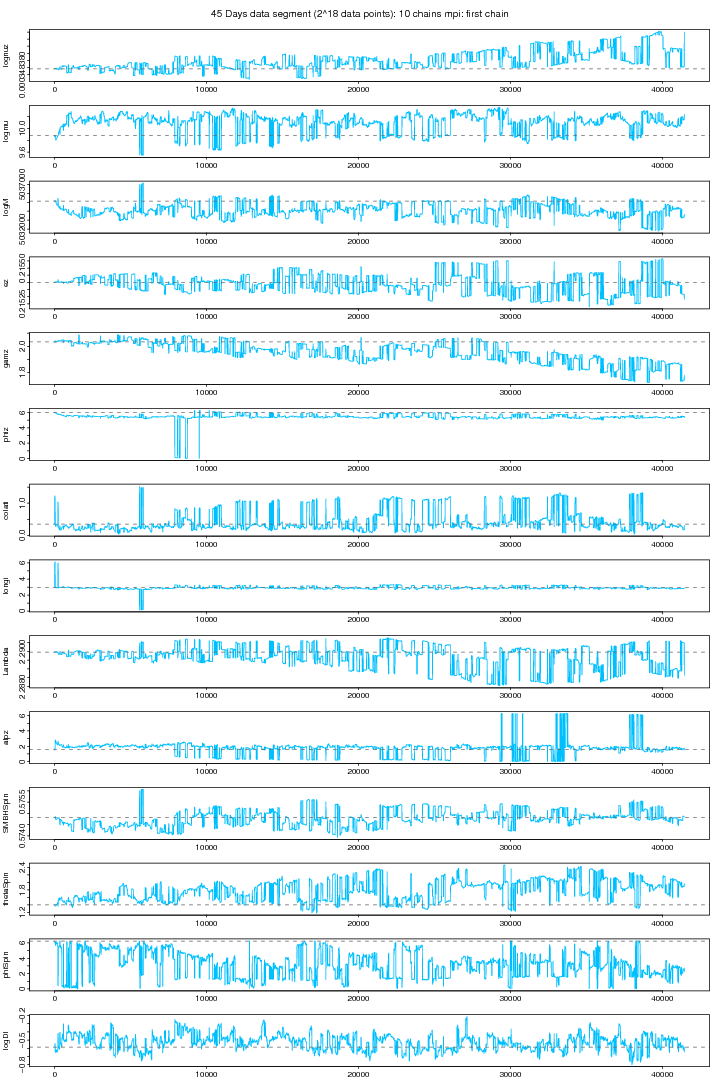
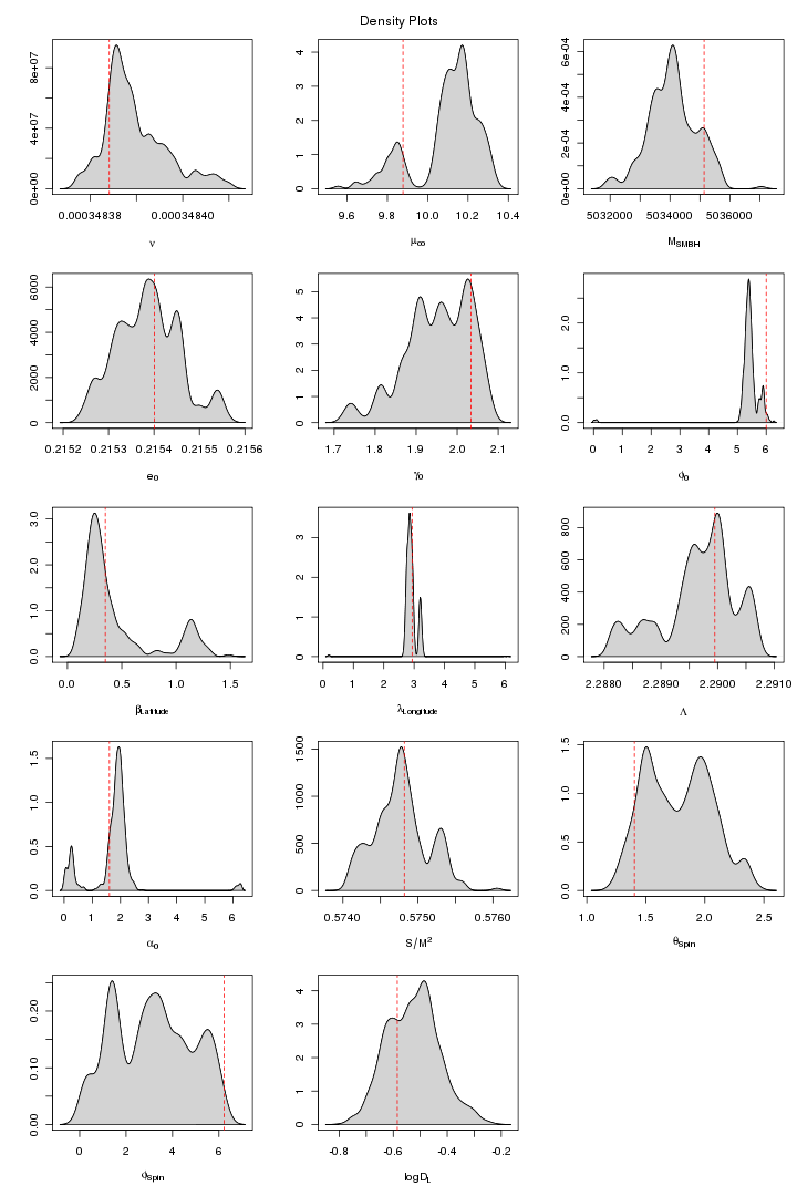
Figure 4. MPI: First chain (cold) out of 10 chains. For PDF format click on figure.

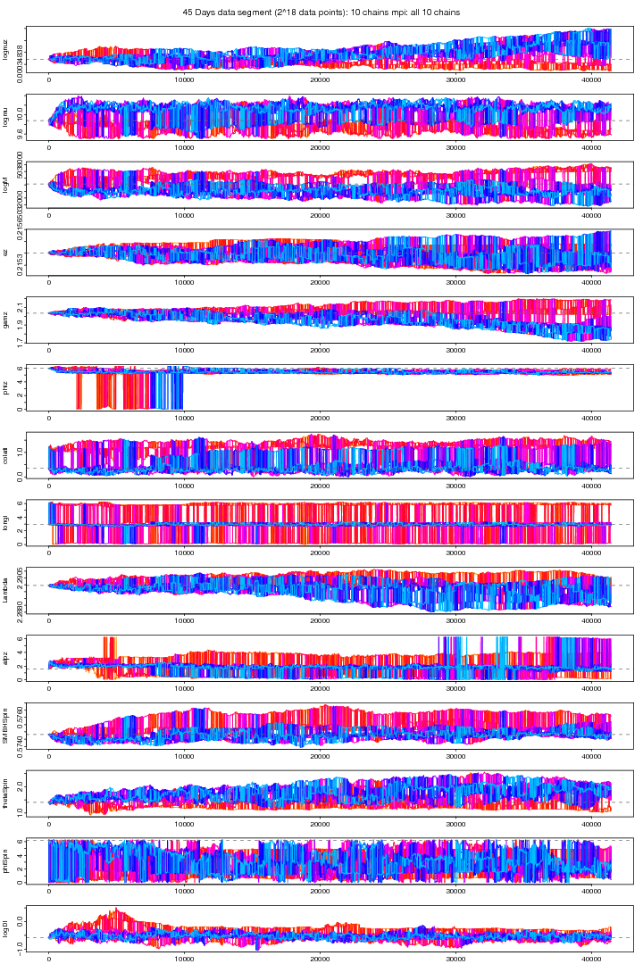
Figure 5. MPI: All the 10 chains. For PDF format click on figure.

The proposal covariance matrix was updated for the above (figure 4 and 5) MCMC by finding the new covariance matrix for the first 10000 iterations. However the new covariance matrix was not positive definite because some of the elements are beyond the tolarance of SETGMN function (used for the generation of multivariate normal deviates in randlib.c). As we are using very small steps particularly for "Orbital Frequency" to keep it in agreement with other parameters (a SD of 1.e-9 works good for it otherwise EMRI are not generated even if generated, takes too long a time and the code takes longer time on that particular iteration and this probably makes our Proposal Covariance Matrix non-positive definite. The first (cold) and all the 10 chains are plotted in figure 4a and 5a. This MCMC trial is still running and till this moment a 10000 iterations were run.

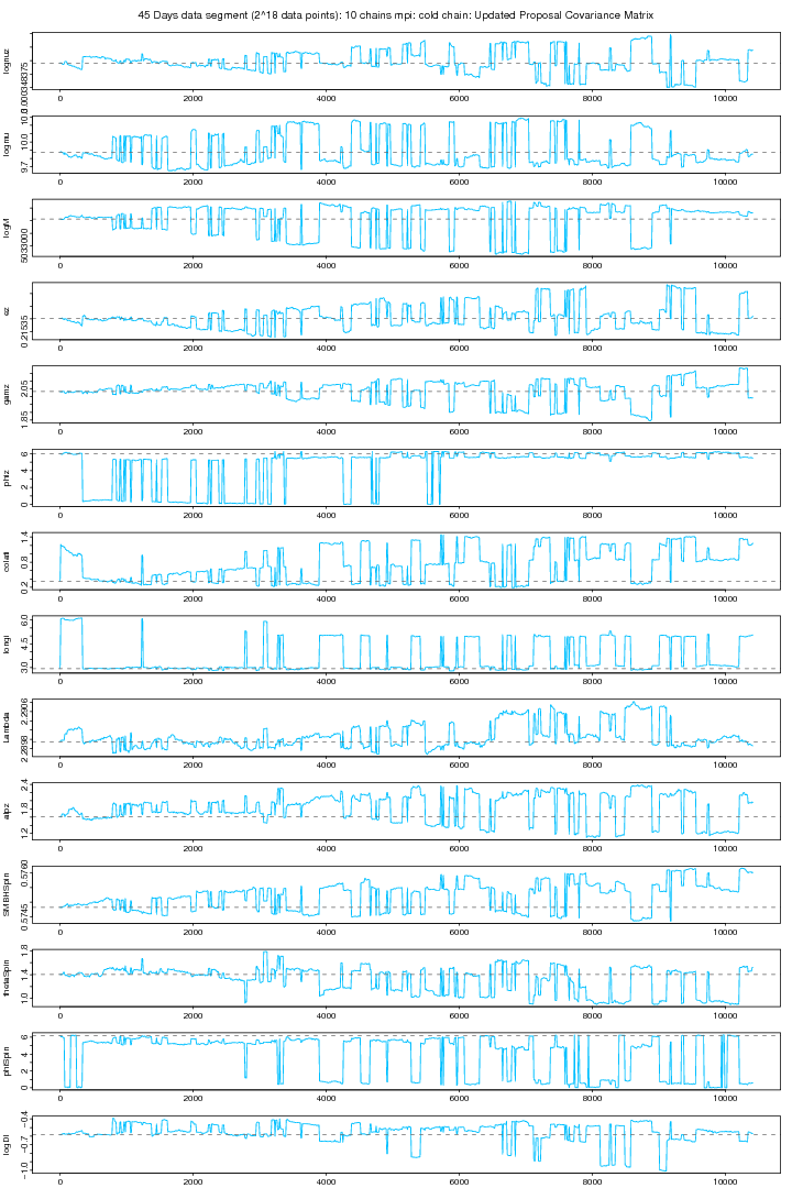
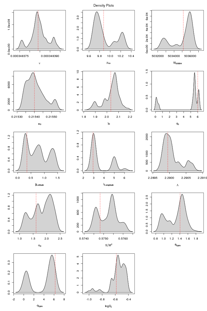
Figure 4a. 10 Chains MPI: First (cold) chain (Updated Covariance). For PDF format click on figure.

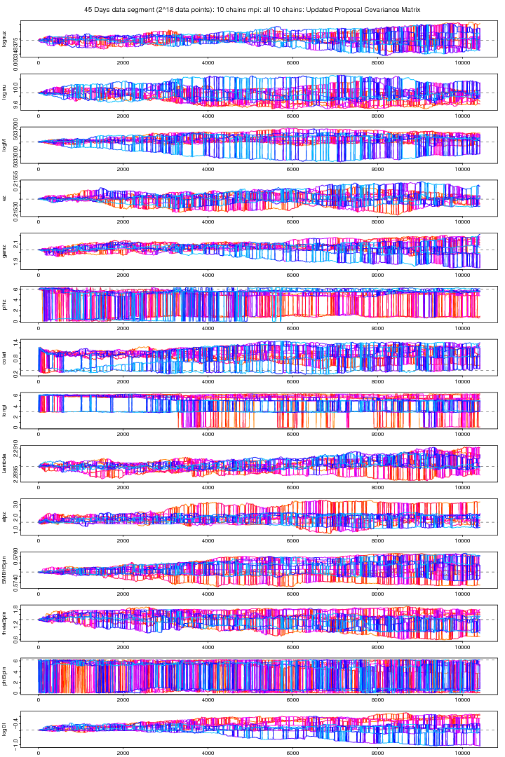
Figure 5a. MPI: 10 Chains MPI: All 10 chains (Updated Covariance). For PDF format click on figure.

One year data: 2²¹ data points

NON-MPI Results

The following two figures (6 and 7) show the plots non-mpi version of MCMC chains run for 5000 iterations over a one year long data set. None of these plots shows any stability.

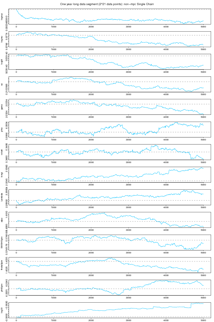
Figure 6. NON-MPI: Chain plot. For PDF format click on figure.

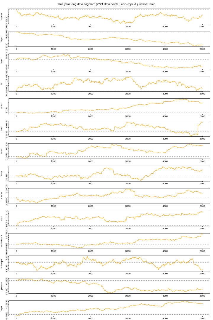
Figure 7. NON-MPI: Hot Chain plot. For PDF format click on figure.

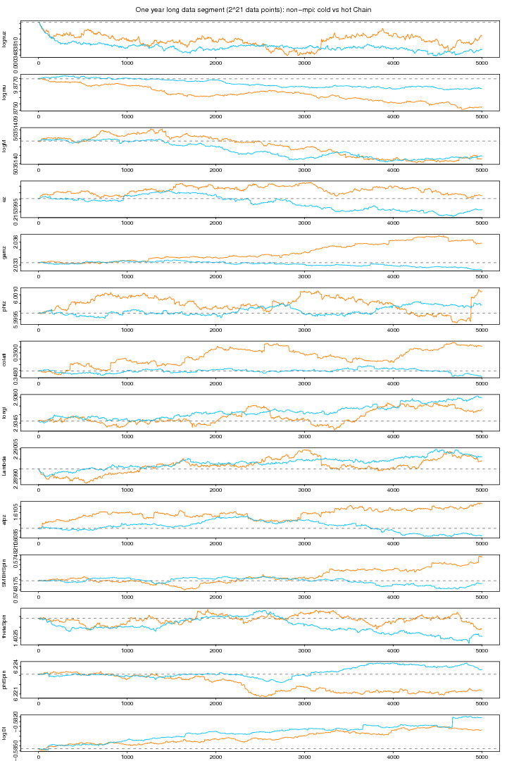
Figure 8. NON-MPI: Cold vs Hot plot. For PDF format click on figure.

MPI Results

The following two figures (9 and 10) show the MCMC chains from MPI version run on 10 chains and a one year long data segment. Figure 9 shows the coldest chain while figure 10 shows all the 10 chains. Except the first parameter ie the orbital frequency no other parameter attains a clear stability.

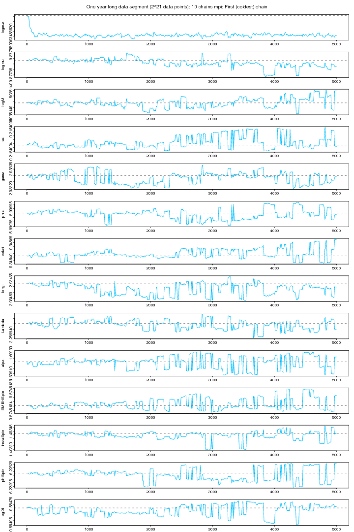
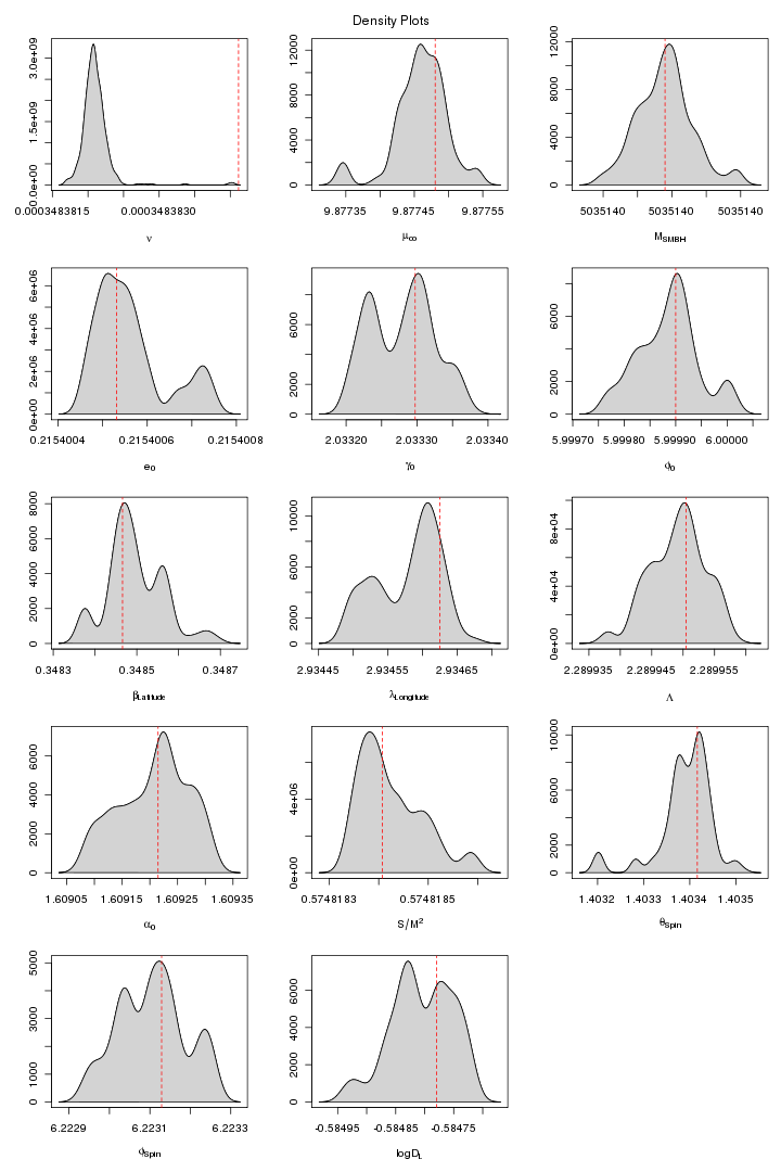
Figure 9. 10 chians MPI: Cold chain plot. For PDF format click on figure.

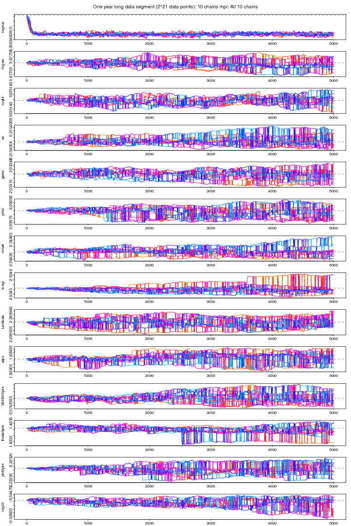
Figure 10. MPI: All 10 chains plot. For PDF format click on figure.

In the following two figures we plot the posterior samples output of a 10 chain parallal tempering MCMC which actually is the continuation of the previous run (figure 9 and 10) in which lognuz (orbital frequency) was converged to a wrong value. Here we set the starting value of lognuz obtained from the last run after discarding the first few hundreds iterations.

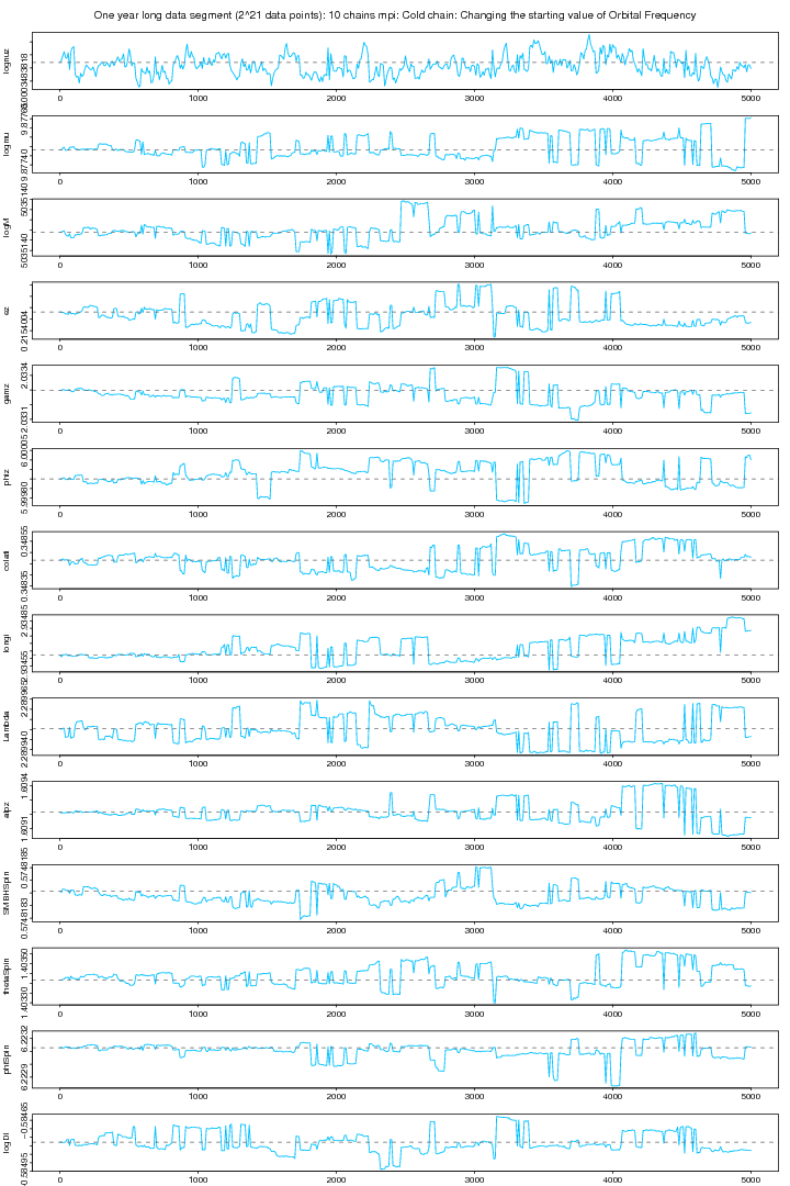
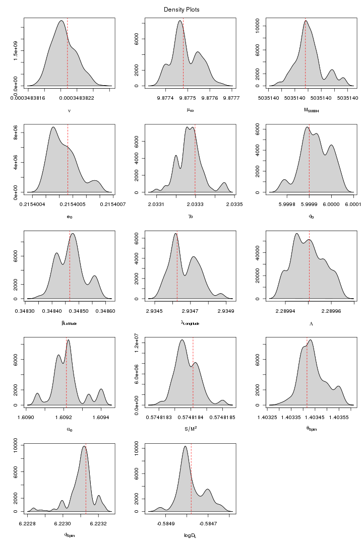
Figure 11. MPI: Cold chain plot after changing the starting value for orbital frequency parameter. For PDF format click on figure.

Here all the 10 chains are plotted and it is evident that all the chains are converged to the same value for lognuz but not for other parameters.

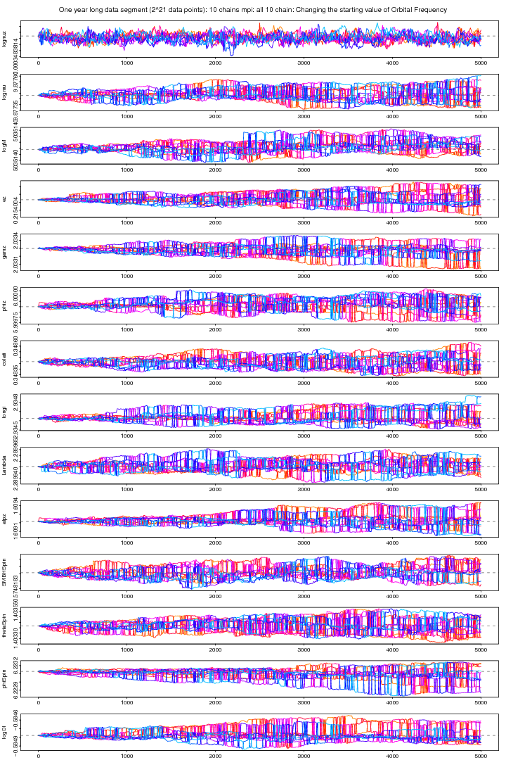
Figure 12. MPI: All 10 chains plot after changing the starting value for orbital frequency parameter. For PDF format click on figure.