|
The name R is used to describe both the R language and the R software environment that is used to run code written in the language.
In this section, we will give a brief introduction to the R software. We will discuss the R language from Section 9.3 onwards.
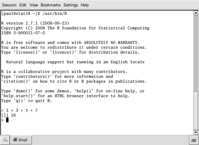
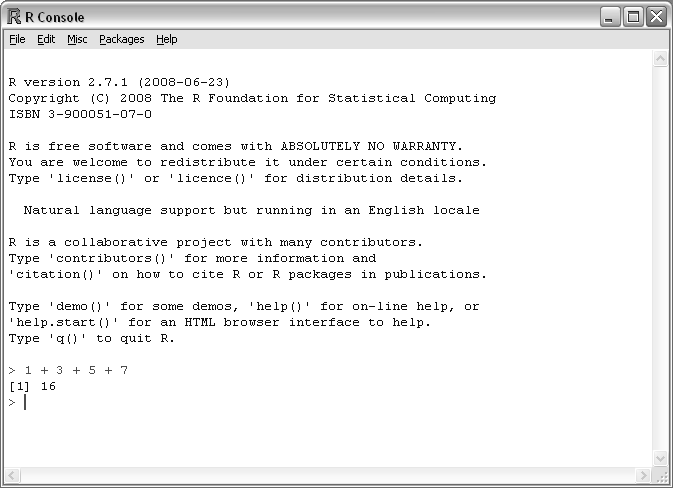
The R software can be run on Windows, MacOS X, and Linux. An appropriate version may be downloaded from the Comprehensive R Archive Network (CRAN).9.1 The user interface will vary between these settings, but the crucial common denominator that we need to know about is the command line.
Figure 9.4 shows what the command line looks like on Windows and on Linux.
|
|
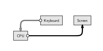
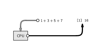
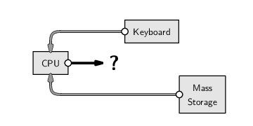
The R command line interface consists of a prompt, usually the > character. We type code written in the R language and, when we press Enter, the code is run and the result is printed out. A very simple interaction with the command line looks like this:
> 1 + 3 + 5 + 7
[1] 16
|
Throughout this chapter, examples of R code will displayed like this, with the R code preceded by a prompt, >, and the results of the code (if any) displayed below the code. The format of the displayed result will vary because there can be many different kinds of results from running R code.
In this case, a simple arithmetic expression has been typed and the numeric result has been printed out.
Notice that the result is not being stored in memory. We will look at how to retain results in memory in Section 9.3.
One way to write R code is simply to enter it interactively at the command line as shown above. This interactivity is beneficial for experimenting with R or for exploring a data set in a casual manner. For example, if we want to determine the result of division by zero in R, we can quickly find out by just trying it.
> 1/0
[1] Inf
|
However, interactively typing code at the R command line is a very bad approach from the perspective of recording and documenting code because the code is lost when R is shut down.
A superior approach in general is to write R code in a file and get R to read the code from the file.
> source("code.R")
|
R reads the code from the file and runs it, one line at a time.
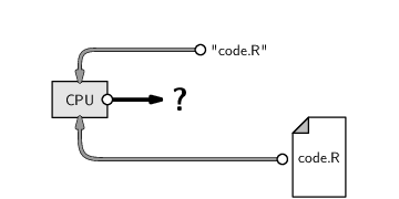
Whether there is any output and where it goes (to the screen, to RAM, or to mass storage) depends on the contents of the R code.
We will look at starting to write code using the R language in Section 9.3, but there is one example of R code that we need to know straight away. This is the code that allows us to exit from the R environment: to do this, we type q().
When quitting R, the option is given to save the “workspace image”.
The workspace consists of all values that have been created during a session--all of the data values that have been stored in RAM.
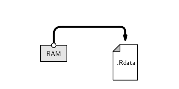
The workspace is saved as a file called .Rdata and when R starts up, it checks for such a file in the current working directory and loads it automatically. This provides a simple way of retaining the results of calculations from one R session to the next.
However, saving the entire R workspace is not the recommended approach. It is better to save the original data set and R code and re-create results by running the code again.
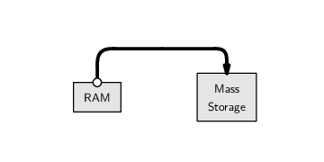
If we have specific results that we want to save permanently to mass storage, for example, the final results of a large and time-consuming analysis, we can use the techniques described later in Sections 9.7 and 9.10.
The most important point for now is that we should save any code that we write; if we always know how we got a result, we can always recreate the result later, if necessary.
The features of R are organized into separate bundles called packages. The standard R installation includes about 25 of these packages, but many more can be downloaded from CRAN and installed to expand the things that R can do. For example, there is a package called XML that adds features for working with XML documents in R. We can install that package by typing the following code.
> install.packages("XML")
|
Once a package has been installed, it must then be loaded within an R session to make the extra features available. For example, to make use of the XML package, we need to type the following code.
> library("XML")
|
Of the 25 packages that are installed by default, nine packages are loaded by default when we start a new R session; these provide the basic functionality of R. All other packages must be loaded before the relevant features can be used.
R code is submitted to the R environment either by typing it directly at the command line, by cutting-and-pasting from a text file containing R code, or by specifying an entire file of R code to run.
R functionality is contained in packages. New functionality can be added by installing and then loading extra packages.
Paul Murrell

This work is licensed under a Creative Commons Attribution-Noncommercial-Share Alike 3.0 New Zealand License.